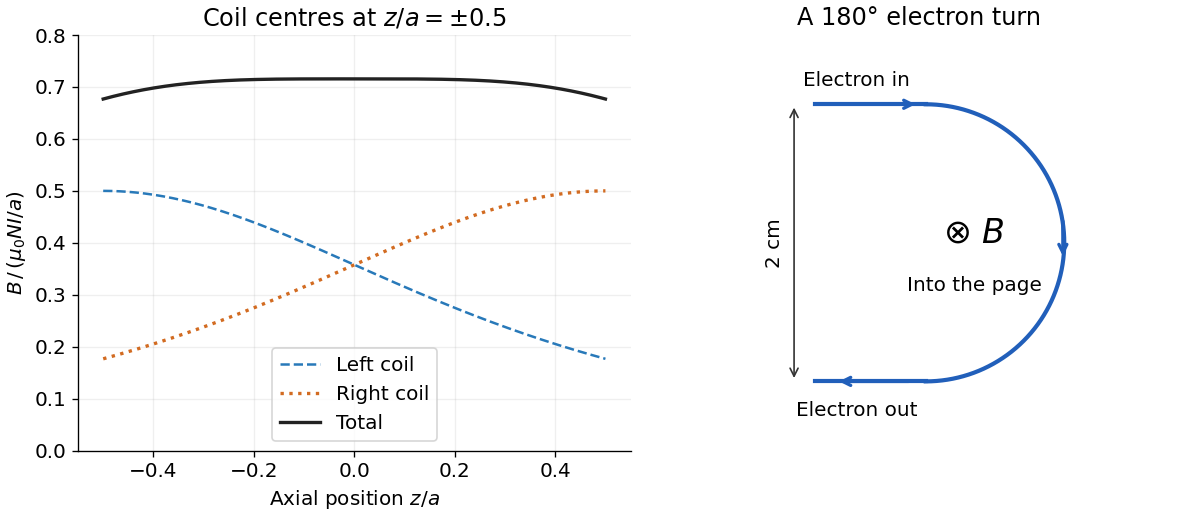
The electron follows a semicircle under the transverse Lorentz force. Parallel, oppositely directed incoming and outgoing paths are separated by a diameter, so the orbit radius is $r=1.00\mathrm{cm}$. Acceleration from rest through the electric potential difference $V$ gives kinetic energy $m_e{v}^2/2=eV$, where $e>0$ is the elementary electric charge. Equating the Lorentz force magnitude to the required centripetal force givesThe magnetic field must be perpendicular to the plane of the turn, with its sign chosen for the electron's negative electric charge. In the illustration the electron enters rightwards at the upper endpoint, so a magnetic field into the page bends it downwards.

The nonrelativistic estimate has $v\simeq 0.198c$. If the small special relativity correction is retained, use $pc=\sqrt{K(K+2m_e{c}^2)}$ with $K=eV$ and $B=p/(er)$. This gives $B\simeq 3.389\times 10^{-2}\mathrm{T}$, about $0.49\%$ larger. The leading answer is adequate at the precision implicit in the classical treatment.

Put the two coil centres at $z=\pm a/2$. By superposition, their axial magnetic field isBoth magnetic field contributions point the same way. Evaluation givesThe corresponding coefficients are $0.715542$ and $0.676777$. Each individual magnetic field falls as one moves away from its own coil; their sum is much flatter near the midpoint.

For a single coil, differentiating $(a^2+x^2{)}^{-3/2}$ twice produces $3(4x^2-a^2)(a^2+x^2{)}^{-7/2}$. At $x=a/2$ this vanishes. Thus the pair has $B^{\prime }(0)=0$ by reflection symmetry and $B^{\prime \prime }(0)=0$ by its chosen separation; all odd derivatives vanish there. In fact,This Helmholtz coil arrangement produces a nearly uniform central magnetic field, useful for controlled charged particle in a uniform magnetic field and magnetic field calibration. The small orbit used below lies within that central region.

For a circular coil, use the Biot-Savart lawAt an axial position $x$, every wire element is at distance $r=\sqrt{a^2+x^2}$. The transverse magnetic field contributions cancel by rotational symmetry. The axial part of $d\mathbf{\ell }\times \mathbf{r}$ is $ad\ell$, and $\oint d\ell =2\pi a$. Multiplying by the $N$ turns givesThe electric current's sense fixes the axial direction by the right-hand rule.

Set the red image at coordinate zero, the blue image at $\delta =0.010\mathrm{m}$, and the screen at $D=1.000\mathrm{m}$. Let the correcting thin lens be at $x$, with $\delta <x<D$. Both original images are then real objects for the correcting thin lens, with positive object distances $u_r=x$, $u_b=x-\delta$, and common positive image distance $v=D-x$. The thin lens equation givesThe refractive indices and Lensmaker's equation requireSubstitute the two focal lengths and cancel $D-x$:Thus the correcting thin lens is $100\mathrm{mm}$ beyond the red image and $900\mathrm{mm}$ before the screen. The required focal lengths and surface radius areThe blue focal length is shorter because the blue refractive index is larger; these two differing object distances are mapped to the same screen, removing the specified longitudinal chromatic aberration.

In the paraxial approximation, apply refraction at each surface of the thin lens in air. With signed radii $R_1$ and $R_2$, the first surface obeys $n/v_1-1/u=(n-1)/R_1$, and the second obeys $1/v-n/v_1=(1-n)/R_2$. The separation of the surfaces is neglected, so the intermediate image coordinate $v_1$ cancels:This is Lensmaker's equation, with Cartesian coordinate system object coordinate $u<0$ for a real object. For an equiconvex thin lens and light travelling left to right, $R_1=R$ and $R_2=-R$. Hence

Electrical contact equalizes electric potential and preserves total electric charge. The usual isolated-sphere approximation assigns the two conducting spheres the capacitances $4\pi {ϵ}_{0}R$ and $8\pi {ϵ}_{0}R$. It then givesThese are accurate when the conducting spheres are far apart and joined by a thin wire. Literal touching changes the answer: each conducting sphere polarizes the other, so its electric potential is not its isolated value. The source does not specify an approximation which would remove this effect.

For completeness, the exact result for ideal externally tangent conducting spheres can be obtained by the method of images. Let their radii be $a,b$, their centre separation $D=a+b$, and their common electric potential $V$. Begin with central image charges $4\pi {ϵ}_{0}Va$ and $4\pi {ϵ}_{0}Vb$. Reflect each external image charge $q^{\prime }$ at centre-distance $s$ into the other conducting sphere of radius $a$: the new image charge is $-a{q}^{\prime }/s$ at centre-distance $a^2/s$ toward the original. Repeat, alternately, in the two conducting spheres. Pairing successive opposite-sign terms gives the convergent net electric chargesEach reflection cancels a nonconstant surface electric potential; the remaining central term fixes $V$. The total internal image charge equals the exterior electric flux divided by $1/{ϵ}_0$, so these sums give the physical net electric charges.

For $a=R,b=2R$, multiply both dimensionless sums by the common factor $4\pi {ϵ}_{0}V(2R/3)$. Their values follow by writing reciprocals as integrals and setting $t=u^3$:Dividing by $S_a+S_b$ enforces conservation of electric charge and yieldsThis concrete touching-sphere result disproves applying the isolated $1:2$ sharing rule to literal contact.

At electrostatic equilibrium the electric field in the metal is zero. The empty cavity also has zero electric field, by the uniqueness theorem for the electrostatic potential. The electric charge lies on the outer surface. For the isolated conducting sphere, spherical symmetry and Gauss's law giveTaking the electric potential to vanish at infinity and using $E_r=-d\varphi /dr$ givesThe electric potential is continuous at the surface, while the normal electric field jumps by $\sigma /{ϵ}_0$, with surface charge density $\sigma =Q/(4\pi R^2)$.

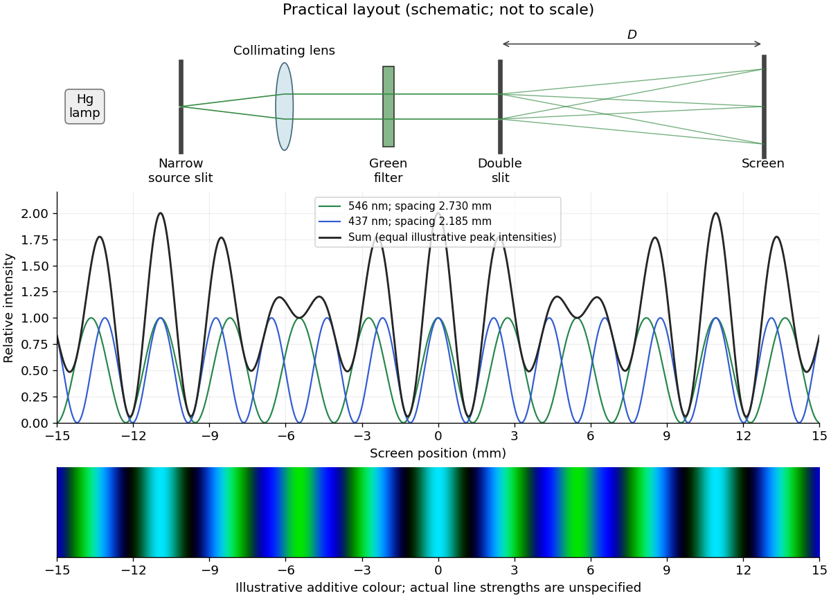
The two wavelengths have independent interference patterns. Their interference fringe spacings areDifferent optical frequencies do not maintain a fixed mutual phase over the detector's integration time, so their intensities add. For narrow equal slits, suppressing the slowly varying diffraction envelopes, one may writeThe relative line strengths are not supplied; the figure illustrates equal peak intensities rather than inferring a quantitative brightness ratio. At $y=0$ both colours are bright, producing a blue-green mixture. Away from the centre the green and blue interference fringes progressively separate, creating alternating colour and brightness variations; places where one line is dark can still be bright in the other. Neither two-line mixing nor its central maximum is generally white.

Across $-15\mathrm{mm}\le y\le 15\mathrm{mm}$, the green maxima occur at $y=2.730m\mathrm{mm}$ for $m=-5,\dots ,5$, and the blue maxima at $y=2.185n\mathrm{mm}$ for $n=-6,\dots ,6$. Near $y=\pm 10.92\mathrm{mm}$, the fourth green and fifth blue maxima nearly coincide: $4{\beta }_g=10.920\mathrm{mm}$ and $5{\beta }_b=10.925\mathrm{mm}$. The $5\mu \mathrm{m}$ mismatch shows that these are near coincidences, not exact ones for the given wavelengths. The plotted central interval includes all these maxima.

Illuminate a narrow entrance slit with the mercury-vapor lamp, use a collimating lens to illuminate two parallel narrow slits coherently, and insert a bandpass filter selecting the green line. Place a screen or scanning detector a measured distance $D$ beyond the double slit. The source slit and the two apertures should be parallel. The aperture widths should be appreciably smaller than their separation to provide an extended diffraction envelope; the green filter should reject the other strong mercury lines. The layout is drawn below.

For slit separation $d$ and observation angle $\theta$, the optical path difference in air is $\Delta =d\sin \theta$. At a bright interference fringe, $\Delta =m\lambda$. For a distant screen and small angles, $\sin \theta \simeq \tan \theta \simeq y/D$, givingMeasuring several interference fringe spacings and dividing by their number reduces relative position error. The derivation assumes the slits have equal phase on illumination and that the screen region lies within their common diffraction envelope.

A mercury-vapor lamp is an extended, spontaneously emitting source, so practical interference requires spatial filtering and spectral selection. A narrow illuminated source slit gives sufficient spatial coherence; selecting one strong spectral line improves temporal coherence and avoids overlapping differently spaced interference fringes.

In the classical double-slit experiment, both apertures are illuminated by the same narrow source. The arrangement is symmetric, permits direct measurement and adjustment of slit separation, and has equal optical materials in the two paths. Its main drawbacks are low transmitted intensity through narrow apertures, the need for a well-made closely spaced slit pair and alignment, and the finite single-slit diffraction envelope. A broad source washes out interference fringes.

Lloyd's mirror uses the direct wave from a narrow source and the reflected wave, which appears to come from its virtual image behind a plane mirror. It requires only one physical source slit; the mirror can be adjusted to make a small effective source separation without manufacturing a double aperture. Only the direct-reflected overlap region shows interference fringes. Finite mirror size, alignment, surface quality, unequal intensities and the polarization-dependent reflection coefficient can reduce visibility. For the usual grazing reflection from glass, the reflected electric wave acquires approximately a $\pi$ phase shift, so the zero path-difference position is dark rather than the bright central fringe of the symmetric classical double-slit experiment. Both arrangements still require adequate spatial coherence and temporal coherence.

The passive RC low-pass filter is simple, inexpensive, requires no power supply, and has no operational amplifier saturation or finite bandwidth limitation. It offers no voltage gain; its output impedance is finite, and both source electrical resistance and loading can change the observed frequency response. Its resistor also produces thermal noise.

The active inverting low-pass amplifier provides a low-frequency voltage gain of magnitude five and, within the usable bandwidth, a small output impedance, so it can drive a load with much less change in frequency response. The input electrical resistance is approximately $R_1=1\mathrm{k}\Omega$ and may itself load the source. It needs a power supply and adds electrical noise and offset; finite operational amplifier gain, bandwidth, slew rate, available output swing, and output electric current limit the ideal formula. Its inversion must also suit the application. The best choice depends on required voltage gain, source and load electrical impedances, and the signal's frequency and amplitude.

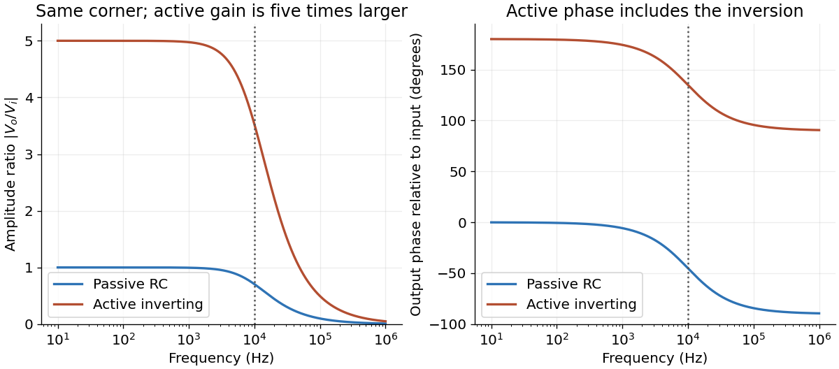
For an ideal operational amplifier under negative feedback, the grounded non-inverting terminal makes the inverting terminal a virtual ground, and no electric current enters either input. The feedback resistor and capacitor have parallel electrical impedanceKirchhoff's current law at the inverting node gives ${\tilde{V}}_i/R_1+{\tilde{V}}_o/Z_f=0$, and henceWith the stated components, $R_{2}C=16.0\mu \mathrm{s}$ and $R_2/R_1=5$. Thus this inverting low-pass amplifier has exactly the same ideal cutoff frequency and normalized frequency response as the passive RC low-pass filter, with output multiplied by $-5$:Its amplitude ratios at the three stated frequencies are $4.99975$, $3.52616$, and $0.97560$. One principal choice of phase shift is $180^{\circ }-{\tan }^{-1}(\omega \tau )$: respectively $179.424^{\circ }$, $134.848^{\circ }$, and $101.252^{\circ }$. Adding or subtracting $360^{\circ }$ describes the same output; the extra inversion must be retained.

Use complex phasors with time dependence $e^{i\omega t}$ and assume an unloaded output. The capacitor has electrical impedance $Z_C=1/(i\omega C)$. The voltage divider formed with the resistor gives the transfer functionFor input $V_i(t)=V_{i0}\cos \omega t$, the output amplitude and phase shift areso $V_o(t)=|{\tilde{V}}_o|\cos (\omega t-{\tan }^{-1}(\omega RC))$.

Here $\tau =RC=16.0\mu \mathrm{s}$, and the cutoff frequency is $f_c=1/(2\pi RC)=9.947\mathrm{kHz}$. This is an RC low-pass filter: at small frequency the capacitor has large electrical impedance and the output nearly equals the input; at large frequency it increasingly shunts the signal to ground. The amplitude then falls as $1/f$, and the phase shift approaches $-90^{\circ }$.

No numerical input amplitude is supplied, so the output voltages are specified as fractions of $V_{i0}$. An application is suppression of high-frequency electrical noise on a slowly varying signal. A finite load changes the transfer function and must be included if its electrical impedance is comparable with the circuit's output electrical impedance.

At the terminal velocity, the acceleration in iii vanishes. ThusFor $0<\varphi <\pi /2$ and nonzero $B$, the magnetic drag increases linearly with speed and this terminal state is stable. Horizontal rails have no gravitational drive. Vertical rails have no linked vertical magnetic flux change, so the model gives free fall rather than a finite terminal velocity.

Project Newton's second law down the slope. The normal reaction has no component along the rails, while the magnetic term opposes motion:This first-order linear differential equation has the release-from-rest solutionThe electrical self-inductance has been neglected; retaining it introduces a coupled electric current equation rather than this instantaneous resistive response.

The component of magnetic force along the slope has magnitude $IBs\cos \varphi$. The rate at which the sliding bar does work against this magnetic braking isBy Ohm's law, $\mathcal{E}=IR$, soThis exactly equals the Joule heating in the resistor in the negligible-self-inductance approximation. The normal force does no work because it is perpendicular to the velocity.

The gravitational power is instead $mgv\sin \varphi$. By the work-energy theorem,It equals the Joule heating only at constant speed. For a concrete counterexample, during the initial acceleration the kinetic energy increases, so some gravitational power remains mechanical.

Use the coordinates in 8. At downhill speed $v$, the moving bar has $\mathbf{v}\times \mathbf{B}=-Bv\cos \varphi \hat{\mathbf{b}}$. The electromotive force and induced electric current are thereforeHere $I$ is positive along $-\hat{\mathbf{b}}$ across the sliding bar, then returns through the rails and resistor. This direction makes the magnetic force oppose downhill motion, as required by Lenz's law. The factor $\cos \varphi$ is essential: only the component of magnetic field normal to the rail plane threads the circuit. Rail and bar electrical resistances and circuit self-inductance are neglected relative to the stated large $R$ model.

For an inductor, $V=Ld{I}_L/dt$. In the steady AC solution with no added constant electric current,The electric current lags the voltage by $\pi /2$. An ideal inductor can also sustain an arbitrary DC current, fixed by initial conditions; it is excluded from this steady sinusoidal comparison.

For a capacitor, $I_C=CdV/dt$, soThe electric current leads the voltage by $\pi /2$.