First use the usual idealization of a grounded infinite conducting plane at $z=0$, with the real point charge $+q$ at $(0,0,d)$. The method of images replaces the metal, for purposes of calculating the exterior electric field, by an image charge $-q$ at $(0,0,-d)$. The exact electric potential in $z>0$ isIt vanishes on the plane, and the uniqueness theorem for the electrostatic potential identifies it with the physical exterior solution. The tangential electric field cancels on the plane, while the normal components add:The electric field inside the conductor is zero, so the electrostatic boundary condition gives $\sigma ={ϵ}_0{E}_z(0^{+})$. Integrating the surface charge density over the facing plane yieldsThe exact image expression is essential near the charge: using the far-field electric dipole approximation at $\rho$ comparable with $d$ would be invalid.

Electrical boundary condition. The source does not specify grounding or the initial total electric charge of the slab. The boxed total is the grounded infinite-plane answer and the large-plane approximation to the charge on its nearby face. An initially neutral, finite, electrically isolated slab retains zero total electric charge; an approximately $-q$ accumulation near the real charge is then balanced by approximately $+q$ on its remote face and edges. This gives a concrete counterexample to interpreting $-q$ as the unconditional total charge of every large metal slab. The local image formula assumes the infinite-plane limit with no applied background electric field.

Apply the negative gradient to the leading far-field electric potential. In spherical coordinates,The electric field therefore has the coordinate-independent formFor the electric dipole along $z$, use $V=\alpha z/(x^2+y^2+z^2{)}^{3/2}$. Direct partial differentiation gives the vector componentsOn the positive axis the electric field points along the electric dipole moment; in the equatorial plane it points oppositely, providing a useful sign check.

The electric dipole moment is $\mathbf{p}=2aq\hat{\mathbf{z}}$. By the superposition principle, the exact electric potential isFor $a/r\ll 1$, the binomial expansion gives each reciprocal distance as $r^{-1}(1\pm (a/r)\cos \theta +O(a^2/r^2))$. The leading $1/r$ terms cancel because the total electric charge is zero. The next even terms also cancel between the two signs. ConsequentlyThis is the leading electric dipole term of the multipole expansion; it describes the far field, not the electric potential arbitrarily close to either point charge.

Keep the source diagram's topology: the arm from the left supply node to $X$ contains $R_0$ and $C_0$ in series; the arm from $X$ to the right supply node is $C_1$; the arm from the left node to $Y$ is $R_1$; and the arm from $Y$ to the right node contains $R$ and $C$ in parallel. Their complex impedances areFor this capacitor bridge with series loss and a parallel standard arm, the detector carries no electric current at balance. Taking the right supply node as zero electric potential and the left one as the source voltage $V_s$, the two voltage dividers give $V_X=V_s{Z}_1/(Z_0+Z_1)$ and $V_Y=V_s{Z}_p/(R_1+Z_p)$. Equality of these complex voltages means equality at every time, rather than merely equality of their magnitudes. Cross multiplication yields $R_1{Z}_1=Z_0{Z}_p$. ThusEquating real and imaginary parts givesThe two adjustable standards determine the two components of the unknown complex impedance. Treating the lower-right arm as a series combination would give a different and incorrect balance equation for the source circuit. The result also gives the dimensionless dielectric loss tangent $\omega C_0{R}_0=\omega RC$ for the series-loss model.

Assume a passive linear electrical circuit in sinusoidal steady state, with transients absent and $V_0$ the peak voltage. Write $Z=|Z|e^{i\varphi }=R+iX$. The electric current is $I(t)=I_0\cos (\omega t-\varphi )$, with $I_0=V_0/|Z|$. Average the instantaneous electric power $V(t)I(t)$ over a full period. The double-frequency term averages to zero, leavingThereforeEquivalently, root mean square values give $⟨P⟩=V_{\mathrm{rms}}{I}_{\mathrm{rms}}\cos \varphi$. The reactance exchanges stored electric field or magnetic field energy with the source, whereas the real part produces Joule heating. A purely imaginary complex impedance dissipates no mean electric power under these ideal assumptions.

For a linear element in sinusoidal steady state, the complex impedance is the ratio of the voltage phasor to the electric current phasor, $Z=\tilde{V}/\tilde{I}$. Use the convention that the physical signal is the real part of its phasor times $e^{i\omega t}$. Then time differentiation becomes multiplication by $i\omega$.

For a resistor, Ohm's law gives $\tilde{V}=R\tilde{I}$. For a capacitor, $I=C\dot{V}$ gives $\tilde{I}=i\omega C\tilde{V}$. For an inductor, $V=L\dot{I}$ gives $\tilde{V}=i\omega L\tilde{I}$. HenceThe imaginary part encodes the relative phase of electric current and voltage: electric current leads voltage in an ideal capacitor and lags it in an ideal inductor.

Neglect fringing field near the edges of the parallel-plate capacitor. Put the plates at $z=0,d$, with prescribed electric potentials $V_A,V_B$. Translational symmetry parallel to a plane makes the electrostatic potential independent of the coordinates parallel to the plates. Thus Laplace's equation reduces to $d^{2}V/d{z}^2=0$. Its general solution is $V=A+Bz$, and the two boundary conditions determine both constants:The electric field is uniform and points toward decreasing electric potential. No plate voltages are specified, so a numerical electric potential cannot be fixed; choosing one plate as the reference only fixes the arbitrary additive constant.

Gauss's law states that the outward electric flux through a closed surface is the enclosed electric charge divided by the vacuum permittivity:In electrostatics, the electric field is the negative gradient of the electrostatic potential, $\mathbf{E}=-\nabla V$. Substitution into the differential equation form of Gauss's law gives Poisson's equation ${\nabla }^{2}V=-\rho /{ϵ}_0$. Consequently, in a region containing no charge density,which is Laplace's equation. Charges on the bounding conductors enter through the boundary conditions; they need not vanish for Laplace's equation to hold inside the empty gap.

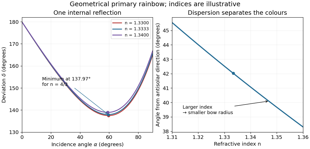
With the Sun behind the observer and raindrops ahead, the one-reflection branch sends many light rays toward directions close to the minimum deviation angle. Nearby values of the angle of incidence produce nearly the same outgoing direction there, forming a wave caustic. For water the resulting cone is approximately $42^{\circ }$ from the antisolar direction. The observer sees the intersecting drops as a circular rainbow, or the part of that circle visible above the ground.

Normal dispersion makes the refractive index larger for violet than for red light. At the minimum, increasing the refractive index increases the deviation angle, and therefore decreases the viewing angle $\pi -{\delta }_{\min }$. Red is on the outer edge of the primary rainbow, violet on the inner edge. The internal specular reflection is partial: with $n=4/3$, the relevant $\beta \simeq 40.2^{\circ }$ is below the critical angle $\arcsin (1/n)\simeq 48.6^{\circ }$. Diffraction and the finite angular size of the Sun smooth the geometrical concentration; the physical intensity does not actually become infinite.

Square the stationary condition and eliminate the angle of incidence using Snell's law:Rearranging yields $3n^2{\sin }^2\beta =4-n^2$. Taking the positive root for a physical incident light ray,An interior minimum exists for $1<n<2$, which includes water at visible wavelengths. For illustration, $n=4/3$ gives $\beta =40.20^{\circ }$, $\alpha =59.39^{\circ }$ and ${\delta }_{\min }=137.97^{\circ }$. The corresponding angle from the antisolar direction is $180^{\circ }-{\delta }_{\min }=42.03^{\circ }$. At $n=2$ the stationary solution reaches the endpoint, and for $n>2$ the displayed square root is not real; the water result is not a formula for every possible refractive index.

Regard the refraction angle as a function of the angle of incidence, $\beta =\arcsin (\sin \alpha /n)$. Implicit differentiation of Snell's law gives ${\beta }^{\prime }=\cos \alpha /(n\cos \beta )$. Differentiating the deviation angle gives ${\delta }^{\prime }=2-4{\beta }^{\prime }$. An interior stationary point therefore satisfiesThe stationary deviation of a primary rainbow ray is a minimum: differentiating $\cos \alpha =n\cos \beta {\beta }^{\prime }$ again and using Snell's law gives ${\beta }^{\prime \prime }=\tan \beta (({\beta }^{\prime }{)}^2-1)$. At the stationary point, ${\beta }^{\prime }=1/2$, and hence ${\delta }^{\prime \prime }=-4{\beta }^{\prime \prime }=3\tan \beta >0$ for a positive interior refraction angle. This minimum is responsible for the concentration of emerging light rays near the primary rainbow direction.

Follow the branch of a light ray that undergoes one internal specular reflection in the spherical drop. At entry, refraction turns its direction by $\alpha -\beta$. The internal specular reflection turns it by $\pi -2\beta$, because the radius is the normal vector and the incidence and reflection angles are both $\beta$. At exit the second refraction contributes another $\alpha -\beta$. Thus the total deviation angle isSnell's law at entry gives $\sin \alpha =n\sin \beta$, taking the surrounding air's refractive index as one. The same internal angle at successive encounters follows from the isosceles triangles formed by each chord and the two radii. Internal specular reflection here need not be total internal reflection; the transmitted branch at that encounter does not belong to the one-reflection trajectory.

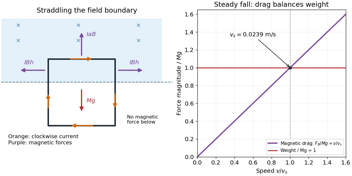
At terminal velocity, the upward magnetic force balances the weight. Substitute the electric current from the preceding solution:The geometric factors cancel, givingHere $g=9.81\mathrm{m}{\mathrm{s}}^{-2}$, $B=1\mathrm{T}$, ${\rho }_m=8960\mathrm{kg}{\mathrm{m}}^{-3}$ and ${\rho }_c=1.7\times 10^{-8}\mathrm{\Omega }\mathrm{m}$. As numerical checks, the specified $a=0.08\mathrm{m}$ and $d_w=0.001\mathrm{m}$ give $M=2.252\times 10^{-3}\mathrm{kg}$, $R=6.926\times 10^{-3}\mathrm{\Omega }$ and $I_s=0.276\mathrm{A}$.

The gravitational power lost, $Mg{v}_s$, equals the Joule heating $I_s^{2}R$, consistent with energy conservation. This terminal velocity applies only while the top arm remains in the magnetic field; after it exits, the magnetic braking ceases, apart from any brief inductive transient.

Use $d\mathbf{F}=Id\mathbf{\ell }\times \mathbf{B}$ for the magnetic Lorentz force on each wire segment. Let $+x$ point right, $+y$ upward and $+z$ out of the page, so $\mathbf{B}=-B\hat{\mathbf{z}}$. With clockwise electric current, the four magnetic forces areThe upper side carries electric current to the right and experiences an upward force, opposing the fall. The bottom side lies outside the magnetic field and has no magnetic force. On the right side the electric current is downward and the force is outward to the right; on the left it is upward and the force is outward to the left. Each side's in-field vertical length is $h$, so these horizontal forces cancel in the net force on the loop.

The wire's total mass is $M=4a{\rho }_m{A}_w$. Uniform wire gives each side a downward weight $Mg/4$. Internal mechanical forces at the corners transmit the unequal loads and maintain the assumed square shape; they cancel for the loop as a whole. The total external vertical force is therefore $Mg-IaB$ downward.

Write the wire diameter as $d_w$ to distinguish it from other geometric labels. Its cross-sectional area is $A_w=\pi d_w^2/4$, and the total wire length is $4a$. From the electrical resistivity, its electrical resistance isWhile the loop straddles the boundary, let $h$ be the height of each vertical side remaining in the magnetic field. The linked magnetic flux has magnitude $Bah$, with $\dot{h}=-v$. Faraday's law therefore gives $|\mathcal{E}|=Bav$. Neglecting the loop's self-inductance, Ohm's law givesThe into-page magnetic flux is decreasing, so Lenz's law requires a clockwise electric current as viewed in the diagram. If the loop is wholly inside a uniform magnetic field, or wholly outside it, its magnetic flux is constant and this induced electromotive force is zero. During a rapid transient one should instead solve $L\dot{I}+RI=Bav$; at the assumed steady speed the same boxed relation holds.

Faraday's law of induction states that the induced electromotive force around a material electrical circuit equals the negative rate of change of its linked magnetic flux:The surface orientation and direction around its boundary are related by the right-hand rule. Lenz's law supplies the physical meaning of the minus sign: the induced electric current produces a magnetic field opposing the change in linked magnetic flux. For a stationary contour the local form is $\nabla \times \mathbf{E}=-{\partial }_t\mathbf{B}$; for this moving wire, the magnetic Lorentz force term is also needed in the electromotive force.

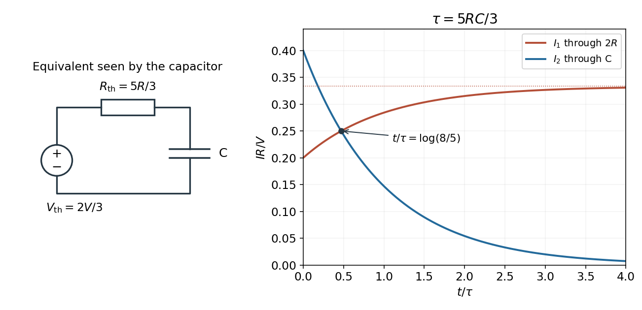
At equality, $I_1=V/(3R)-I_2/3=I_2$, so the common electric current is $V/(4R)$. Substituting the capacitor electric current givesThereforeFor $R=50\mathrm{k\Omega }$ and $C=0.2\mathrm{microfarads}$, $RC=0.0100\mathrm{s}$ and $\tau =0.01667\mathrm{s}$, giving $\boxed{t\simeq 7.83\mathrm{ms}}$. The battery electric potential difference cancels, as expected because every electric current scales linearly with it in this ideal linear circuit. The result assumes a nonzero source electric potential difference; with $V=0$ both electric currents vanish at all times.

Kirchhoff's current law at the left capacitor terminal gives $(V-V_a)/R=V_a/(2R)+I_2$. Since $I_1=V_a/(2R)$,Thus $I_1$ rises from $V/(5R)$ to $V/(3R)$, whereas $I_2$ falls from $2V/(5R)$ to zero. Their derivatives have opposite signs, and both approach their limiting values on the same time scale $\tau =5RC/3$. The graph uses electric currents in units of $V/R$ and time in units of $\tau$.

Label the capacitor's left terminal $a$ and right terminal $b$, with the battery's negative node at zero. The source diagram has $2R$ from $a$ to ground, $R$ from $b$ to ground, and a source-side resistor $R$ feeding $a$ from electric potential difference $V$. The capacitor electric current $I_2$ flows from $a$ to $b$; $I_1$ flows through $2R$.

With the capacitor removed, $V_a=2V/3$ and $V_b=0$, so the Thévenin equivalent seen by the capacitor has $V_{\mathrm{th}}=2V/3$. Suppress the ideal electric potential difference source to find its electrical resistance: the left terminal sees $R\parallel 2R=2R/3$ to ground and the right sees $R$, giving $R_{\mathrm{th}}=5R/3$ between the terminals.

The initially uncharged capacitor electric potential difference $V_C=V_a-V_b$ therefore obeysSolving gives $V_C=(2V/3)(1-e^{-t/\tau })$, with $\tau =R_{\mathrm{th}}C$. The capacitor electric current is $I_2=C{\dot{V}}_C$, henceAt $t=0^{+}$, the short-like uncharged capacitor makes $V_a=V_b=2V/5$, so $I_2=2V/(5R)$ directly from the right resistor. At long times the capacitor carries no direct electric current. These endpoint checks agree with the exponential solution.

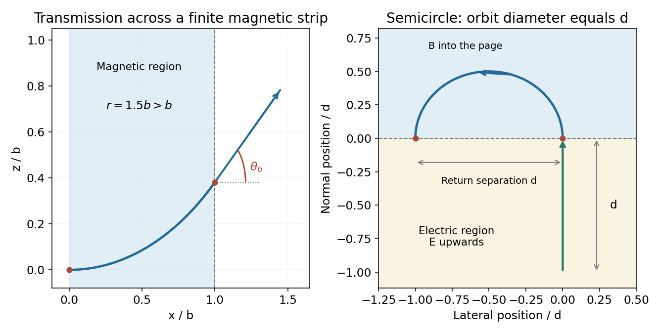
The electric field does work $qEd$ on the initially stationary particle. Thus the entry speed into the magnetic region isIn the source geometry the magnetic field is perpendicular to the page, and the particle enters perpendicular to the straight interface. Its return to that interface occurs after a semicircle. The separation between exit and return points is its orbit diameter, so the required separation $d$ gives $r=d/2$. ConsequentlyFor the drawn field into the page and a positive charge entering upwards, the trajectory bends left. Its speed is constant while in the magnetic field, so the time there is the semicircle length divided by $v_0$:The last form is half the cyclotron period and independently checks the geometric calculation.