Topics (384k) Articles (398k) Users (410) Discussions (242) Comments (383) Files (13k) New article
Past exam of the kinetic theory course of the University of Oxford 2025 3 e Solution by  Codex 0 2026-10-25
The required time separation is , where is the evolution timescale of , together with and an observation time well after the pulse. The first condition permits freezing at its pre-pulse value; its neglected change would enter beyond the retained second order. The second makes the original initial time lie in a negligible tail of the Gaussian function, permitting replacement of the lower time limits by . Short duration alone would not justify that replacement for a pulse centered at the initial time.
Integrate the continuity equation in c over the whole pulse. For fixed , the time factor is the ordered Gaussian response integralA common translation by removes the peak time. Pair the positive and negative azimuthal harmonics: is paired with . Both and change sign, so their product does not; makes the two time factors complex conjugates. Hence the pair contributes .
For completeness, the real part of the integrand is symmetric under . The triangular time domain therefore gives half of the full plane, and the Fourier transform of a Gaussian function givesThis derives the supplied identity rather than requiring a separate time-ordering calculation.
DefineUsing the paired harmonics and now yieldsBy the stated assumption, is independent of , so its exponential can be taken outside the radial integral. Put and useThereforeThe outer derivative acts on the Gaussian resonance broadening factor as well as on the radial integral. The result describes quasilinear diffusion in action space weighted by the squared pulse amplitude, with a detuning width . A shorter pulse has broader frequency selectivity, while a longer pulse selects narrower orbital resonances. If the action-space boundary flux vanishes, integrating over gives zero, as required by conservation of mass.
Past exam of the kinetic theory course of the University of Oxford 2025 3 d Solution by Codex 0 2026-10-25
Codex 0 2026-10-25The restriction describes an -fold rotating perturbation of a galactic disk, for example a transient spiral density wave or, for , a galactic bar. Its pattern speed is , its amplitude peaks at , and its Gaussian function envelope has duration of order . The coefficients describe its strength along different stellar orbits. A real perturbing potential requires .
Past exam of the kinetic theory course of the University of Oxford 2025 3 c Solution by Codex 0 2026-10-25
Codex 0 2026-10-25Let denote . Average the Collisionless Boltzmann equation to second order. All first-order angle derivatives average to zero, leavingAn angle integration by parts shows thatThus the angle-averaged galactic distribution function obeys an action-space continuity equation,This sign also follows from Hamilton's equations, : the flux is .
Reality gives and . Orthogonality of the Fourier series impliesInsert b to obtainAlthough individual terms are complex, pairing with makes the flux real.
Now take the marginalization specified by . Assume vanishing radial-action flux at and : the first boundary does not permit negative radial action, and the second has no escaping flux in this calculation. ThenwithIf radial-action boundary flux were present, its explicit boundary term would have to be retained.
Past exam of the kinetic theory course of the University of Oxford 2025 3 b Solution by Codex 0 2026-10-25
Codex 0 2026-10-25Use the Collisionless Boltzmann equation in action-angle variables,Define the orbital frequency vector byThe slow evolution of the angle average starts at second order in the perturbation. At first order, the Poisson bracket therefore givesFor the th term in the Fourier series, this readsThe lowercase here denotes the Fourier coefficient of the uppercase in the Hamiltonian; these are the same perturbing potential. Multiply by the integrating factor and set the initial homogeneous response to zero. One obtainsRetaining the slow time dependence of inside this integral is compatible with the subsequent second-order calculation; changes in caused by that slow evolution affect only higher orders in this approximation.
Past exam of the kinetic theory course of the University of Oxford 2025 3 a Solution by Codex 0 2026-10-25
Codex 0 2026-10-25For a regular integrable Hamiltonian system, action-angle variables offer two related simplifications.
- Unperturbed Hamilton's equations are and . Complicated stellar orbits become uniform motion on an invariant torus, and the unperturbed transport operator becomes . A Fourier series in the angles then makes orbital resonances explicit through .
- A phase-mixed equilibrium galactic distribution function depends on the action variables rather than the fast angles, consistently with Jeans theorem. Its slow evolution, including quasilinear diffusion in action space, can therefore be described by an angle average in two action variables rather than by resolving every stellar orbit in position and velocity.
These advantages assume regular or approximately integrable mean motion; globally defined action-angle variables need not exist in chaotic regions.
Past exam of the kinetic theory course of the University of Oxford 2025 2 f Solution by Codex 0 2026-10-25
Codex 0 2026-10-25For , the upper Langmuir wave starts at and approaches the line from above. The lower Langmuir wave starts at and approaches from below. The electron acoustic wave starts at the origin with slope and approaches from above; it stays inside . These are the only completely undamped branches, as shown by the cubic equation in b.
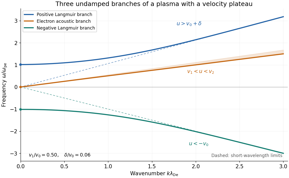
The small asymmetry between the outer branches reflects the extra positive-velocity population introduced by the velocity plateau. The negative- sketch follows by rotating the displayed branches through the origin, since on these undamped solutions. One should not impose symmetry about the axis at fixed positive .
Past exam of the kinetic theory course of the University of Oxford 2025 2 e Solution by Codex 0 2026-10-25
Codex 0 2026-10-25Retain while making the same narrow-velocity plateau expansion as in d. With , the factor that varies rapidly across the plateau is . The other factors vary slowly and may be evaluated at , givingThereforeAt , the denominator tends to , recovering d. At ,recovering the exponentially close approach to the plateau edge in c. The phase velocity remains strictly inside the velocity plateau for every finite .
As an asymptotic expansion, the formula takes at fixed . If the plateau also approaches the outer edge, so that is comparable to , the factors treated as slowly varying need not be slowly varying. In that additional limiting regime, use the exact dispersion relation in b instead.
Past exam of the kinetic theory course of the University of Oxford 2025 2 d Solution by Codex 0 2026-10-25
Codex 0 2026-10-25For the two outer branches, at small . An integration by parts and a large- expansion giveThere is no boundary contribution because the phase-space distribution function vanishes at both endpoints. Direct area integration givesThus the exact small- cutoff, retaining the paper's definition , is . To leading order in the narrow-velocity plateau approximation this isThese are Langmuir waves. The difference between and the reference is only first order in , so it does not alter the requested leading-order result.
For the finite-phase velocity branch put , with . To leading order in and , the real dispersion relation becomesAt long wavelength set to leading order. Then , andFor comparison, the exact phase velocity from the cubic equation in b is ; expanding it gives precisely at fixed .
A single Maxwell-Boltzmann velocity distribution has a nonzero slope at every finite nonzero and has no velocity plateau. The would-be electron acoustic wave is therefore subject to strong Landau damping, so there is no corresponding completely undamped acoustic branch in a single Maxwellian electron population with immobile ions. At its only stationary point , a Maxwellian has , making the static dielectric function positive rather than zero. This statement does not exclude acoustic modes of suitably distinct electron populations or an ion-supported mode when ion dynamics is retained.
Past exam of the kinetic theory course of the University of Oxford 2025 2 c Solution by Codex 0 2026-10-25
Codex 0 2026-10-25For , the logarithm in b must be large and positive. In each allowed interval this happens near a denominator zero, approached from the undamped side:The constants hidden by have velocity units. Consequently,The two outer modes have phase velocities just outside the occupied range and therefore have no resonant particles. The middle electron acoustic wave lies just inside the lower edge of the velocity plateau, where . All three escape Landau damping in this collisionless model. The stated neglect of ion response remains necessary for the middle mode as well.
Past exam of the kinetic theory course of the University of Oxford 2025 2 b Solution by Codex 0 2026-10-25
Codex 0 2026-10-25Let , , and . Use the Debye length convention of the paper, . On the candidate intervals in a, the Landau contour contributes no imaginary part. The piecewise constant slopes giveSince , setting the dielectric function to zero yieldsThe absolute values express the real response on the allowed intervals. Solving this real equation inside a sloping portion of would not satisfy the imaginary part of the dielectric function.
An exact algebraic form will also make the number of undamped branches clear. DefineOn each allowed interval, the quantity inside the logarithm equals . Exponentiating and usinggives the cubic equationFor every , the logarithm runs from to on , from to on , and from to on . The intermediate value theorem supplies a root in each interval, and the cubic equation permits at most three. Thus there is exactly one undamped branch in each interval.
Past exam of the kinetic theory course of the University of Oxford 2025 2 a Solution by Codex 0 2026-10-25
Codex 0 2026-10-25Take initially; real solutions for follow by . Put . Approaching the real phase velocity from the upper half-plane, the Landau contour and the Sokhotski–Plemelj formula give the following Cauchy principal value decompositionThe real frequency condition therefore requires . This is possible in the interior of the velocity plateau and outside the occupied velocity range:These are candidate intervals, not yet solutions of the real dispersion relation. The endpoints have jumps in and logarithmic singularities in the response; they are not finite- undamped modes. At the cusp , the slope is also discontinuous and the real response diverges, so it supplies no additional mode.
The physical condition is absence of net resonant energy exchange with particles moving at the wave's phase velocity. Outside the support there are no such particles. Within a velocity plateau, the equal populations on either side of the resonance cancel Landau damping.
Past exam of the kinetic theory course of the University of Oxford 2025 1 d Solution by Codex 0 2026-10-25
Codex 0 2026-10-25Write and introduce the raw third velocity moment and the third central velocity moment :The expansion of their product givesThe heat flux is for unit mass.
Multiply the BGK model by . The external force term isTherefore the raw second velocity moment satisfiesThe matching local Maxwellian has , soTo remove the bulk motion, let be the material derivative. The continuity equation and the momentum conservation equation implyand henceSubtract this identity from the raw second velocity moment equation and insert the expansion of . The terms and cancel by the product rule. The external force terms also cancel, since a common acceleration changes the local mean velocity without directly changing the relative velocities. What remains isThe trace of the relaxation term is zero because . Thus the BGK model relaxes anisotropy of the pressure tensor while preserving the local random kinetic energy. The evolution is still a velocity-moment hierarchy, since requires further information about .
Past exam of the kinetic theory course of the University of Oxford 2025 1 c Solution by Codex 0 2026-10-25
Codex 0 2026-10-25Use the BGK model from b. Multiply it by and integrate over velocity space. Matching the collision invariants makes the collision contribution vanish. For the external force term, integration by parts givesDefine the momentum flux and force density byThe resulting momentum conservation equation isThe pressure tensor is the second central velocity moment,The zeroth velocity moment also supplies the continuity equation , which will be needed in d.
Past exam of the kinetic theory course of the University of Oxford 2025 1 b Solution by Codex 0 2026-10-25
Codex 0 2026-10-25To obtain the Boltzmann equation, take a dilute gas with a short-range pair potential. Its interaction range is small compared with the mean free path and the spatial scale on which the phase-space distribution function changes. The binary collision approximation treats encounters as isolated elastic collisions; simultaneous encounters involving three or more particles can be neglected. The encounter duration is short compared with the collision relaxation time and macroscopic evolution time, and the external force changes negligibly during an encounter. This permits local, effectively instantaneous scattering at one position .
The essential statistical closure is molecular chaos for the Boltzmann equation: the distribution of incoming pairs factorizes as . Outgoing pairs need not be independent. Follow each incoming pair through its two-body scattering, and use conservation of momentum and kinetic energy, together with time reversal and the invariant scattering measure, to express both gain and loss in the same variables. This givesHere ; when the measure is written as , its Jacobian is included in the Boltzmann scattering kernel. In a scattering-angle convention, that kernel contains relative speed times differential scattering cross-section. The hemisphere prevents double counting equivalent outcomes for indistinguishable particles; the precise factor is included in . The primed velocities are connected to the unprimed ones by the reversible elastic collision map. This closure is appropriate for a dilute short-range gas, rather than a generic long-range interacting system with an important collective mean-field theory contribution.
The further replacement by the BGK model is a phenomenological relaxation closure. Replace the full nonlinear Boltzmann collision operator by relaxation towards a local Maxwellian, with a single, velocity-independent collision relaxation time :It models relaxation towards a local Maxwellian without resolving the detailed scattering. Treating as constant is an additional simplification; it is of the order of a mean time between effective collisions. Near a local Maxwellian, departures in the nonconserved velocity moments decay on this timescale.
Choose to match the collision invariants , and of . For unit particle mass, this meansHere is the mass density, is the mean velocity, and is the temperature in squared-velocity units, before setting . In particular,Thus relaxation preserves local mass, momentum and kinetic energy rather than relaxing them to externally prescribed values.
Past exam of the kinetic theory course of the University of Oxford 2025 1 a Solution by Codex 0 2026-10-25
Codex 0 2026-10-25Normalize the symmetric -particle phase-space distribution function to one and write , . The number-normalized one- and two-particle distribution functions areThus and . These conventions absorb the otherwise explicit factor in the first BBGKY hierarchy equation.
Separate the Hamiltonian into kinetic energy, external potential energy, and pair potential terms. Their Hamilton's equations giveThe sign follows directly from the stated Poisson bracket: . The Hamiltonian Liouville equation is consequentlyIntegrate over and multiply by . Assume sufficient decay in velocity space and either decay or periodic boundary conditions in position, so that integration by parts removes all transport terms with . The surviving interaction term iswhere indistinguishability makes all terms equal. Relabeling as yields the exact resultNo assumption of molecular chaos for the Boltzmann equation has entered: the dependence on the two-particle distribution function is still exact.
Past exam of the kinetic theory course of the University of Oxford 2024 3 f Solution by Codex 0 2026-10-25
Codex 0 2026-10-25With and from e, inversion givesFor , deform the contour downwards. Closing below is clockwise, so the residue theorem multiplies the sum of enclosed residues by . The forcing pole has residue and therefore contributesA simple collective root of the continued gravitational dielectric function contributesThese are the Landau mode transients excited by introducing the mass abruptly. For a strictly damped background they decay, together with any remaining phase-mixing contour contribution under the usual regularity and decay assumptions. ThusThe causal boundary value is what the paper abbreviates by . Physically, the moving mass polarizes the stellar population and carries a gravitational wake. Each spatial harmonic is changed in amplitude and phase by at the forcing frequency. Self-gravity can amplify the wake. The induced part alone is ; the wake's back-reaction on the perturber produces dynamical friction.
The waiting time is controlled by the slowest excited collective damping, not just an orbital or crossing time. If with , then a modal amplitude is suppressed by , and one needs for every appreciably excited mode, together with decay of the phase-mixing remainder. Large transient prefactors can require additional time. Near marginal stability, a relevant tends to zero and the required waiting time diverges; the stationary wake approximation is then not uniform in the stability parameter.[ref]
The linear response of stellar systems does not diverge at marginal stability by Chris Hamilton and Tobias Heinemann. Sections 2.1–2.2: forcing-pole and Landau-mode contributions, and the nonuniform late-time limit
Qualification of stability. If stable means only non-growing, a persistent neutral mode invalidates the asserted asymptote. A concrete example is a homogeneous waterbag distribution with parallel marginal . Its gravitational dielectric function isFor , the roots are real, so the switch-on transients persist although that harmonic has no growing mode. Taking the smallest box wavenumber to satisfy the same inequality makes the whole waterbag model free of growing harmonics. The claimed late-time formula therefore requires damping of all excited modes and ; exact forcing at an undamped root instead produces a secular response.
Past exam of the kinetic theory course of the University of Oxford 2024 3 e Solution by Codex 0 2026-10-25
Codex 0 2026-10-25Represent the perturber by the periodic Dirac delta function at . With spatial Fourier series coefficient normalized by , its nonzero density coefficients areThe mean density is subtracted as in d. The Poisson equation for Newtonian gravity givesThe perturbation is zero before switch-on. For , its Laplace transform isHenceThe switch-on creates a forcing pole at the real frequency , approached causally from the original upper inversion contour.
Past exam of the kinetic theory course of the University of Oxford 2024 3 d Solution by Codex 0 2026-10-25
Codex 0 2026-10-25In the periodic cube, , so . The supplied action-angle variables are canonical: . For ,Consequently c becomesFor each nonzero wavenumber, the Poisson equation for Newtonian gravity givesSubstitute the preceding response and add the externally imposed Newtonian gravitational potential:ThereforeThis gravitational dielectric function has the opposite susceptibility sign to the electron dielectric function, reflecting attractive rather than repulsive collective interactions. The homogeneous mean field is explicitly subtracted in this fictitious periodic model: the Poisson equation for Newtonian gravity acts on density fluctuations, and the mode is omitted. Otherwise a nonzero uniform positive mass density would be incompatible with a periodic potential. This is the convention often called the Jeans swindle.
For analytic continuation, resolve velocity parallel to : let and . ThenStart at and deform the Landau contour continuously below the moving pole. At real , the integral isFor , this causal continuation equals the undeformed real-axis integral plus wherever has the necessary analytic extension. It must not be replaced by the undeformed integral alone.
Zeros of are self-consistent collective Landau modes: with no external forcing, a nonzero Newtonian gravitational potential is possible at such a root. For time dependence , upper-half-plane roots grow, lower-half-plane roots describe Landau damping, and real roots are neutral. Damped Landau modes are poles of the continued response; they need not be regular discrete eigenfunctions of the original collisionless operator.
Regularity qualification. Continuation throughout the complex plane presupposes suitable analytic . Arbitrary smooth need not allow it. For example, for and zero elsewhere is smooth but not analytic at ; its Cauchy integral cannot be holomorphically continued across those endpoints. The Landau contour gives the standard causal continuation on the domains where the equilibrium permits it, with possible singularities retained.
Past exam of the kinetic theory course of the University of Oxford 2024 3 c Solution by Codex 0 2026-10-25
Codex 0 2026-10-25Use the stated Fourier series normalization, so . Then b givesFor the Laplace transform with kernel , integration by parts yieldsThe upper boundary vanishes for sufficiently large , and the initial term is zero by hypothesis. ThusorThe denominator identifies the orbital resonance between the perturbation and unperturbed orbital frequencies. The zero harmonic has no driving term and remains zero with these initial data.
Past exam of the kinetic theory course of the University of Oxford 2024 3 b Solution by Codex 0 2026-10-25
Codex 0 2026-10-25Since and depend only on the action variables, . Drop the quadratic term from the Vlasov equation in a. Defining the orbital frequency vector by , the linearized equation isThe sign of the driving term follows from the second term in the canonical Poisson bracket, because the background has no angle dependence.
Pinned article: Introduction to the OurBigBook Project
Welcome to the OurBigBook Project! Our goal is to create the perfect publishing platform for STEM subjects, and get university-level students to write the best free STEM tutorials ever.
Everyone is welcome to create an account and play with the site: ourbigbook.com/go/register. We belive that students themselves can write amazing tutorials, but teachers are welcome too. You can write about anything you want, it doesn't have to be STEM or even educational. Silly test content is very welcome and you won't be penalized in any way. Just keep it legal!
Intro to OurBigBook
. Source. We have two killer features:
- topics: topics group articles by different users with the same title, e.g. here is the topic for the "Fundamental Theorem of Calculus" ourbigbook.com/go/topic/fundamental-theorem-of-calculusArticles of different users are sorted by upvote within each article page. This feature is a bit like:
- a Wikipedia where each user can have their own version of each article
- a Q&A website like Stack Overflow, where multiple people can give their views on a given topic, and the best ones are sorted by upvote. Except you don't need to wait for someone to ask first, and any topic goes, no matter how narrow or broad
This feature makes it possible for readers to find better explanations of any topic created by other writers. And it allows writers to create an explanation in a place that readers might actually find it.
Figure 1. Screenshot of the "Derivative" topic page. View it live at: ourbigbook.com/go/topic/derivativeVideo 2. OurBigBook Web topics demo. Source. - local editing: you can store all your personal knowledge base content locally in a plaintext markup format that can be edited locally and published either:This way you can be sure that even if OurBigBook.com were to go down one day (which we have no plans to do as it is quite cheap to host!), your content will still be perfectly readable as a static site.
- to OurBigBook.com to get awesome multi-user features like topics and likes
- as HTML files to a static website, which you can host yourself for free on many external providers like GitHub Pages, and remain in full control

Figure 2. You can publish local OurBigBook lightweight markup files to either OurBigBook.com or as a static website.
Figure 3. Visual Studio Code extension installation.
Figure 5. . You can also edit articles on the Web editor without installing anything locally. Video 3. Edit locally and publish demo. Source. This shows editing OurBigBook Markup and publishing it using the Visual Studio Code extension. 
- Infinitely deep tables of contents:



All our software is open source and hosted at: github.com/ourbigbook/ourbigbook
Further documentation can be found at: docs.ourbigbook.com
Feel free to reach our to us for any help or suggestions: docs.ourbigbook.com/#contact