Topics (384k) Articles (398k) Users (410) Discussions (242) Comments (383) Files (13k) New article
Past exam of the kinetic theory course of the University of Oxford 2024 3 a Solution by  Codex 0 2026-10-25
For an integrable or approximately integrable background Hamiltonian, action-angle variables turn an otherwise complicated stellar orbit into and . This has two useful consequences. First, a phase-mixed equilibrium can be represented directly as : the action variables label the unperturbed orbits, while angle variables describe position along them. Second, the angles are periodic, so Fourier series reduce unperturbed transport to multiplication by and make orbital resonances explicit. The action variables also separate rapid orbital motion from slow secular changes. These advantages apply on regular orbital regions; a globally chaotic background need not admit global action-angle variables.
The transformation is canonical, preserving the phase space measure and the stated total mass . The collisionless Vlasov equation isHere is the single-star specific Hamiltonian; the normalization of by mass changes neither the Poisson bracket nor the transport equation.
Past exam of the kinetic theory course of the University of Oxford 2024 2 e Solution by Codex 0 2026-10-25
Codex 0 2026-10-25The long-wavelength limit in d is resonant heating. Most electrons screen the slowly varying spatial field. The noise nevertheless excites collective Langmuir waves, whose sharp temporal spectrum lies near . Electrons with remain in phase with a wave and exchange energy with it. A stable tail absorbs net wave energy through Landau damping. The heating is initially deposited in narrow tail regions of velocity space, even though the volume-integrated rate equals that in c.
The short-wavelength limit in c is stochastic heating in the terminology intended here. With , the imposed electric field is essentially unscreened. Its temporally uncorrelated kicks cause a random walk of electron velocity, so . Electrons throughout the thermal population contribute to the resulting kinetic energy increase; no narrow collective wave peak selects a small tail population.
Both mechanisms are driven by white noise, and the formal condition enters the stationary quasilinear diffusion calculation in both cases. The physical distinction is the sharp collective resonance in d versus the broad direct random forcing in c, rather than the mere presence of randomness. In collisionless theory this heating is an increase of the averaged kinetic energy; subsequent collisions can establish thermal equilibrium.
Past exam of the kinetic theory course of the University of Oxford 2024 2 d Solution by Codex 0 2026-10-25
Codex 0 2026-10-25Set and first work with a representative positive . For , the thermal core is strongly screened. However, the causal dielectric function has weakly damped Langmuir wave roots , with , and . Their phase velocities are in the tail. Both roots must be retained for each spatial Fourier series harmonic.
Write . The supplied approximation givesExpanding to first order gives the Landau damping rateIn particular, stable damping means . Near either root,The narrow Lorentzian resonance approximation then gives the leading resonant contributionThis is a formula under the integral over velocity; it is not a pointwise approximation away from the resonances. Insert it into the heating formula in c. For one spatial harmonic, the contribution from one root isbecauseThus the tiny tail slope cancels the tiny Landau damping rate: weak absorption is compensated by a large noise-driven wave intensity. The two temporal roots supply two equal halves of the answer. Negative gives the same result by the conjugate response of a real electric field, without altering the original convention that the spatial sum includes both signs. ThereforeAs in c, equality means the leading result in the stated asymptotic limit. This calculation assumes nonzero damping, observation times , and forcing weak enough that changes negligibly during that relaxation. Taking zero damping before the long-time limit invalidates the stationary calculation.
Past exam of the kinetic theory course of the University of Oxford 2024 2 c Solution by Codex 0 2026-10-25
Codex 0 2026-10-25For a regular thermal and noise at , the susceptibility is small at thermal phase velocities: its scale is . To leading order the electrons cannot appreciably screen such short-scale fields, and b becomes independent of velocity:The electron kinetic energy per unit volume is . Assume and vanish at infinity. One integration by parts gives the general heating formulaFor constant , a second integration by parts and giveThis is the leading short-wavelength result. With vanishing boundary flux, the diffusion equation also conserves particle number; constant conserves the mean momentum while increasing the random kinetic energy.
Past exam of the kinetic theory course of the University of Oxford 2024 2 b Solution by Codex 0 2026-10-25
Codex 0 2026-10-25A linearly stable has no zeros of the causal dielectric function in . Hence the inverse Laplace transform contours can approach , retaining the causal boundary value at . To obtain a stationary forced response, further assume that the excited collective perturbations actually damp. This is the decay condition in the question's long-time instruction.
A transparent evaluation of the double integral uses the stationary power spectral density. The white noise covariance has temporal spectrum . Linear filtering by therefore givesThe causal solution for in a gives, after the initial transients have decayed,The real part can be taken because the full sum pairs conjugates. Using the distribution theory identity , with a positive vanishing convergence factor, samples the temporal spectrum at :The factor from the one-sided time integral cancels the in the noise covariance. The result is nonnegative, as a stationary velocity-space diffusion coefficient should be.
Qualification of stability. Absence of growing modes alone does not guarantee this stationary limit. For example, the electron waterbag distribution hasas undamped collective roots. White noise drives their field variance to grow instead of settling. Thus the formula requires decay of excited modes, not merely absence of exponentially growing ones. For weak Landau damping, the waiting time can be much longer than , and must still be short compared with evolution of for the frozen-background quasilinear approximation to apply.
Past exam of the kinetic theory course of the University of Oxford 2024 2 a Solution by Codex 0 2026-10-25
Codex 0 2026-10-25Use the electron electric charge , so gives acceleration . The Vlasov equation, its average, and its linearized fluctuating part areThe quasilinear approximation retains the averaged quadratic term but drops products of fluctuations from the fluctuating equation. It freezes the slowly evolving during the fast response calculation. A real electrostatic potential has , and the sum includes both signs of every nonzero wavenumber. Spatial averaging selects the opposite Fourier series harmonics; statistical homogeneity supplies the corresponding diagonal noise covariance.
Let . Zero initial givesInsert this into the electrostatic self-consistency relation. Using and givesThis derives the stated dielectric function with the Landau contour. A noise-free growing collective response is a zero of .
The Laplace transform of the white noise covariance is particularly simple. Writing ,For clarity about contour signs, introduce the inverse-transform measuresThe first Bromwich inversion formula contour runs upward on ; its conjugate contour runs downward on . Both measures therefore have the same positive orientation in their real frequency parameters. Combining the averaged equation with yieldsAt a zero of , the last expression means its continuous coefficient obtained before cancelling . Substitution of the two inverse Laplace transforms and the transformed covariance givesThis is the paper's expression, with the orientation of made explicit. Reality follows by pairing and . The double integral retains switch-on transients; replacing it by a time-independent diffusion coefficient requires the additional long-time limit in b.
Past exam of the kinetic theory course of the University of Oxford 2024 1 d Solution by Codex 0 2026-10-25
Codex 0 2026-10-25Spatial homogeneity makes independent of position and makes the two-particle number density depend only on the separation. Isotropy removes its directional dependence. ConsequentlyHere is a radial distribution function, with the finite- normalization inherited from a; statistical independence is unnecessary. In particular, the translated pair in c has separation for every , so its integral is simply .
Isotropy of the random velocity makes its second velocity moment proportional to the identity. Taking its trace fixes the proportionality constant:Thus is the one-component random velocity variance; for unit mass in thermal equilibrium, . A Maxwell-Boltzmann velocity distribution is not required for the pressure tensor to be isotropic.
For the interaction contribution, the angular integral is , by isotropy and its trace. With , c becomesCombining the two pressure tensors gives the virial pressure from pair correlations:For a repulsive pair potential, the outward radial force is . Since , the second term in is nonnegative, and positive when occupied separations feel nonzero repulsion. It expresses additional momentum transfer through interactions. The displayed integral assumes a differentiable pair potential and convergence; a hard core requires a contact formula or a limiting argument.
Past exam of the kinetic theory course of the University of Oxford 2024 1 c Solution by Codex 0 2026-10-25
Codex 0 2026-10-25For fixed and , define with and . The chain rule givesso . The derivative with respect to here translates both arguments of the two-particle number density; it is not a derivative of its first argument alone.
Take the spatial divergence of the proposed interaction pressure tensor. Its pair potential factor is independent of , so the preceding identity givesExchange symmetry of the two-particle distribution function implies . In the second term, substitute . Since is odd, both terms become equal:On the other hand, at fixed , the first-argument derivative of the pair potential is . Thus the interaction force density in b is . Moving it to the left yields local conservation of momentum:The integral over distributes each pair's momentum flux along the straight segment joining the particles. The factor removes the double counting of ordered pairs. Central forces also make .
Past exam of the kinetic theory course of the University of Oxford 2024 1 b Solution by Codex 0 2026-10-25
Codex 0 2026-10-25Take the zeroth velocity moment of a. The right side is a velocity space divergence with vanishing boundary contribution, giving the continuity equationFor the first velocity moment, use integration by parts componentwise:Write ; then , and the momentum flux splits into bulk transport and the pressure tensor:Thereforewhere repeated Cartesian indices are summed and . The negative sign is the attractive or repulsive force , rather than an additional sign convention for the pressure tensor.
Past exam of the kinetic theory course of the University of Oxford 2024 1 a Solution by Codex 0 2026-10-25
Codex 0 2026-10-25Put and . Normalize the symmetric -particle phase-space distribution function to one. Use factorial normalization for its one-particle marginal and two-particle distribution function:Thus and . For unit particle mass, also carries mass density. These conventions explain why no extra factor occurs in the result.
Separate the Hamiltonian as , whereand contains all terms involving only particles . The stated Poisson bracket gives Hamilton's equationsConservation of probability along the Hamiltonian flow gives the Hamiltonian Liouville equationAssume decay of the required velocity moments and either decay or periodic boundary conditions in position. Integrating over eliminates the terms by integration by parts. The terms in differentiating an integrated velocity also vanish. Indistinguishability makes the remaining terms equal, soRelabeling the two particles gives the first BBGKY hierarchy equation:This is exact for a differentiable pair potential; no independent-particle closure has been made.
Past exam of the kinetic theory course of the University of Oxford 2023 3 e Solution by Codex 0 2026-10-25
Codex 0 2026-10-25Apply the chain rule to with :On the resonance selected by the Dirac delta function, . ThusEvery weight is nonnegative, and . Strict positivity additionally requires a populated nonaxisymmetric resonance with nonzero coupling on a set of positive surface measure. The unconditional statement is nonnegativity, rather than positive definiteness. As a concrete counterexample to strict positivity of this formula, retain one nonzero conjugate harmonic pair with and choose its smooth coefficient supported in an open region . The perturbation is nonzero but has zero resonant coupling, so even when . The even simpler zero-perturbation case also gives zero. Whether a particular physical stellar bar has nonzero resonant overlap is additional information.
For a coupled stellar bar and halo, the halo gains positive angular momentum and exerts the opposite torque on the stellar bar. If the halo mass is and the rigid stellar bar has constant positive moment of inertia , thenThis bar-halo angular-momentum transfer is a form of dynamical friction: a resonantly coupled stellar bar tends to slow down while the dark matter halo spins up. Actual long-term evolution changes both the stellar bar pattern and the halo distribution function, so the fixed-pattern response must then be updated. If the stellar bar changes its moment of inertia, the general relation is ; positive moment of inertia alone would not fix the sign of without that rigidity assumption.
Past exam of the kinetic theory course of the University of Oxford 2023 3 d Solution by Codex 0 2026-10-25
Codex 0 2026-10-25Write , , and let the detuning from the rotating perturbation beSubstitute into the linear response in action-angle variables, then set :At exact resonance the last quotient is interpreted by its continuous limit . Inserting this response in c givesPair with . Because , , and , the imaginary cosine terms cancel. The finite-time torque isThis is a leading, second-order response in the perturbation amplitude.
For the long-time limit, assume a continuum of occupied action variables, sufficiently smooth integrable weights, convergent harmonic sums, and regular resonance surfaces wherever a contributing surface intersects the distribution. Assume also that the perturbation is weak enough to neglect nonlinear trapping and secular changes in , and that the prescribed stellar bar pattern and its coefficients stay fixed. Then phase mixing removes nonresonant transients in the integrated response. The relevant long-time resonance kernel is the distributional convergenceIt is not a pointwise limit: at the kernel equals . To justify its use under the integral over action variables, resolve the integral into detuning surfaces; the coarea formula givesSmoothness and decay of this surface weight reduce the limit to the one-dimensional long-time resonance kernel. Equivalently, a causal convergence factor gives as .
Therefore the resonant torque from a rotating perturbation isOnly orbital resonances contribute to this steady integrated torque. The limit is a formal weak-perturbation limit, or an intermediate-time approximation after phase mixing but before substantial secular redistribution. It does not prove an unchanged halo can absorb angular momentum at this rate forever. A discrete set of orbital frequencies, singular resonance surfaces, or strong trapping can invalidate the stated steady limit.
Past exam of the kinetic theory course of the University of Oxford 2023 3 c Solution by Codex 0 2026-10-25
Codex 0 2026-10-25Since , Hamilton's equations giveFor the spherical unperturbed Hamiltonian, ; in these particular action-angle variables the third component describes the fixed orientation of the orbital plane. It should not be confused with the physical azimuthal angular velocity of a particle around its orbit.
The conserved normalization of a probability distribution makes the expected value of specific angular momentum equal to . Its time derivative is the torque per unit halo mass:This follows either by averaging the single-particle equation or by integrating the Collisionless Boltzmann equation against , with vanishing boundary fluxes.
The term integrates to zero over the periodic angle variable. Thus the first nonzero torque is quadratic in the perturbation. Use the Fourier series expansions of b; the source's reference here to part (a) is a numbering slip. Integrating the product over all three angle variables yieldsReality of the potential energy per unit mass gives ; likewise . Conjugate harmonics make the total torque real. The sum is over all integer vectors, so no extra factor of two should be inserted.
Past exam of the kinetic theory course of the University of Oxford 2023 3 b Solution by Codex 0 2026-10-25
Codex 0 2026-10-25Define the unperturbed orbital angular frequency vector byIt is the rate of advance of the angle variables along the unperturbed Hamiltonian flow; the action variables are constant. Expand the Collisionless Boltzmann equation to first order in the perturbations. Since and depend only on the action variables, , andThe omitted Poisson bracket is quadratic in the perturbations. Use the Fourier series conventionFor each harmonic the linear ordinary differential equation isMultiplication by the integrating factor and use of give the causal linear response in action-angle variables:The zero harmonic stays zero at this order. This formula retains the entire forcing history; replacing it immediately by a resonant Dirac delta function would discard the transient response.
Past exam of the kinetic theory course of the University of Oxford 2023 3 a Solution by Codex 0 2026-10-25
Codex 0 2026-10-25The action-angle variables are canonical coordinates, with . In the convention , their Poisson bracket isIn particular, Hamilton's equations read and , fixing the sign needed below.
Past exam of the kinetic theory course of the University of Oxford 2023 2 e Solution by Codex 0 2026-10-25
Codex 0 2026-10-25The two real branches start at , have zero initial slope, and approach the lines from outside the populated parallel-velocity region. The original plot solves the degenerate-plasma dielectric response numerically; the shaded wedge shows where particles with resonant parallel velocities exist.
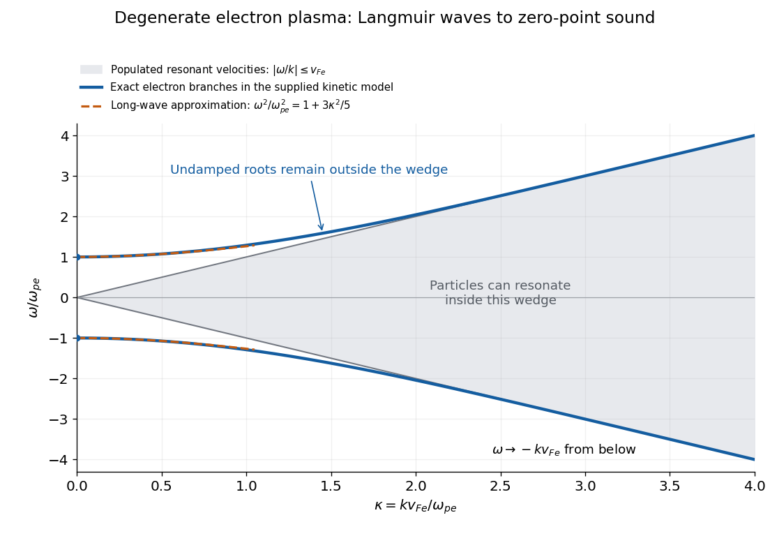
The distinction from a nondegenerate gas with a Maxwellian Maxwell-Boltzmann velocity distribution is its tail. A Maxwellian has resonant particles at every finite phase velocity. Its long-wavelength Langmuir waves have exponentially weak Landau damping, but at shorter wavelengths that damping becomes strong. The ideal degenerate cutoff instead permits this undamped branch to persist continuously into degenerate-plasma zero-point sound. The coefficient in c is also different from the classical thermal dispersive coefficient.
A natural additional branch is a degenerate ion-acoustic wave. For singly charged ions with equal electron and ion number densities, degenerate electron pressure supplies a restoring force while ion mass supplies inertia. The electron equation of state has , suggesting, at long wavelengths,Both species are degenerate here, so . The hierarchy explains the damping: there are no resonant ions, but there are resonant electrons inside their parallel marginal distribution. That electron marginal distribution has a small nonzero slope at , even though the full three-dimensional occupation is constant inside the Fermi sphere. One therefore expects weak electron Landau damping, of relative order , rather than exact absence of damping. Ion degeneracy pressure adds a relatively small correction to . This reasoning concerns an electrostatic ion-acoustic wave; transverse or magnetized branches require additional field dynamics or a background magnetic field.
Past exam of the kinetic theory course of the University of Oxford 2023 2 d Solution by Codex 0 2026-10-25
Codex 0 2026-10-25For the positive-frequency branch write , , and . The degenerate-plasma dielectric response is equivalent toAt large , a logarithmic divergence is needed to balance the right-hand side; hence . Keeping the constant as well as the large term givesMore precisely the relative correction is . The additive constant in the exponent fixes the leading prefactor and should not be discarded.
The negative-frequency branch follows from the even real dielectric function outside the occupied interval. ThusUsing the physical Thomas-Fermi screening length instead gives . This is degenerate-plasma zero-point sound: the phase velocity lies exponentially close to, but strictly beyond, the edge of the Fermi sphere for every finite in this approximation. The limit is a property of the supplied classical-trajectory kinetic theory; applying it at microscopic wavelengths would require checking quantum recoil, which that equation omits.
Past exam of the kinetic theory course of the University of Oxford 2023 2 c Solution by Codex 0 2026-10-25
Codex 0 2026-10-25Let and . The long-wavelength electron branch has . The convergent power seriesturns the degenerate-plasma dielectric response intoSubstitute . The coefficient of is , so the degenerate-plasma Langmuir dispersion isThe Langmuir wave therefore has a finite frequency at zero wavenumber, with the first dispersive correction set by the Fermi velocity. Indeed the occupied Fermi sphere has , so the coefficient agrees with the high-phase velocity velocity moment expansion.
Screening-length convention. The source defines , so its long-wavelength condition is equivalent to . We retain that definition when expressing answers in its symbols. The actual electron Thomas-Fermi screening length obtained from the static response is insteadFor a concrete comparison, at , the static dielectric function is ; using the printed length as the physical Thomas-Fermi screening length would give . Calling the printed length the Debye length thus differs from the physical degenerate-electron screening convention by a factor of three. It does not affect the boxed dimensional dispersion relation.
Past exam of the kinetic theory course of the University of Oxford 2023 2 b Solution by Codex 0 2026-10-25
Codex 0 2026-10-25There is no Landau damping of this branch within the completely degenerate collisionless model. Its phase velocity obeys , while each parallel marginal distribution vanishes outside . There are no particles at the resonant velocity, and . The Landau contour consequently contributes no imaginary part to the dielectric function; a real root is allowed with .
If a small nonzero temperature supplied a tail beyond the Fermi surface, the conclusion would change: the resonant derivative would generally be nonzero. For the convention and a simple weakly damped root, expanding the continued dielectric function would give . This conditional formula is not needed to manufacture damping for the exact cutoff. Neither collisional attenuation nor nonlinear evolution is included in the given dispersion relation.
Past exam of the kinetic theory course of the University of Oxford 2023 2 a Solution by Codex 0 2026-10-25
Codex 0 2026-10-25The step in the source must be at zero. We use the Heaviside step function for , zero for , with its value at zero immaterial here. The printed threshold is inconsistent with both and the stated number density. For example, measuring velocities in fixed units and taking , the literal printed cutoff fills only and gives one eighth of the stated number density. Its distributional derivative is , not . The zero-threshold convention restores the stated Fermi sphere and its normalization of a probability distribution.
Let , choose , and abbreviate . The three-dimensional phase-space distribution function is , whereIntegrate over the transverse velocity disk to obtain the parallel marginal distributionThere are no edge Dirac delta functions in because itself vanishes continuously at the endpoints. In particular, the three-dimensional constant occupation does not imply a constant parallel marginal distribution.
Use time dependence , with and for damping. The given dielectric function becomesThe Landau contour supplies causal continuation. For a real phase velocity , there is no resonant pole in the populated interval, andHence this species contributes
For comparable species number densities and fixed charge ratios, implies and . Since , the ions have and . Their response is negligible to leading order in the mass ratio. The real dispersion relation is thereforeThis degenerate-plasma dielectric response treats a completely degenerate, nonrelativistic Fermi gas with classical particle trajectories. It does not include quantum recoil or a collision term. A finite ion response shifts the root slightly; the boxed equation is the stated leading electron approximation.
Pinned article: Introduction to the OurBigBook Project
Welcome to the OurBigBook Project! Our goal is to create the perfect publishing platform for STEM subjects, and get university-level students to write the best free STEM tutorials ever.
Everyone is welcome to create an account and play with the site: ourbigbook.com/go/register. We belive that students themselves can write amazing tutorials, but teachers are welcome too. You can write about anything you want, it doesn't have to be STEM or even educational. Silly test content is very welcome and you won't be penalized in any way. Just keep it legal!
Intro to OurBigBook
. Source. We have two killer features:
- topics: topics group articles by different users with the same title, e.g. here is the topic for the "Fundamental Theorem of Calculus" ourbigbook.com/go/topic/fundamental-theorem-of-calculusArticles of different users are sorted by upvote within each article page. This feature is a bit like:
- a Wikipedia where each user can have their own version of each article
- a Q&A website like Stack Overflow, where multiple people can give their views on a given topic, and the best ones are sorted by upvote. Except you don't need to wait for someone to ask first, and any topic goes, no matter how narrow or broad
This feature makes it possible for readers to find better explanations of any topic created by other writers. And it allows writers to create an explanation in a place that readers might actually find it.
Figure 1. Screenshot of the "Derivative" topic page. View it live at: ourbigbook.com/go/topic/derivativeVideo 2. OurBigBook Web topics demo. Source. - local editing: you can store all your personal knowledge base content locally in a plaintext markup format that can be edited locally and published either:This way you can be sure that even if OurBigBook.com were to go down one day (which we have no plans to do as it is quite cheap to host!), your content will still be perfectly readable as a static site.
- to OurBigBook.com to get awesome multi-user features like topics and likes
- as HTML files to a static website, which you can host yourself for free on many external providers like GitHub Pages, and remain in full control

Figure 2. You can publish local OurBigBook lightweight markup files to either OurBigBook.com or as a static website.
Figure 3. Visual Studio Code extension installation.
Figure 5. . You can also edit articles on the Web editor without installing anything locally. Video 3. Edit locally and publish demo. Source. This shows editing OurBigBook Markup and publishing it using the Visual Studio Code extension. 
- Infinitely deep tables of contents:



All our software is open source and hosted at: github.com/ourbigbook/ourbigbook
Further documentation can be found at: docs.ourbigbook.com
Feel free to reach our to us for any help or suggestions: docs.ourbigbook.com/#contact