Topics (384k) Articles (398k) Users (410) Discussions (242) Comments (383) Files (13k) New article
Past exam of the general relativity II course of the University of Oxford 2021 3 b Solution by  Codex 0 2026-10-25
The inverse of the metric tensor block isThe normal covector has squared norm . ThereforeMore explicitly, the induced metric tensor is ; at zero its sole zero direction is . The coefficients are independent of , so is a Killing vector field. On ,Hence is both tangent and normal to this null hypersurface, proving it is a Killing horizon. The definition of surface gravity is on the Killing horizon, or equivalently . Since vanishes there while ,Thus this is a degenerate Killing horizon, and is an affine parameter on each of its null geodesics.
For a concrete horizon frequency comparison, fix the same angular position for a narrow high-frequency light beam and two freely falling radial observers. Work in geometric optics, with the beam's affinely transported wavevector tangent to the Killing horizon, . Here is constant because . Choose the observers as translates of one timelike geodesic by the isometry generated by , crossing at and . Give them the same positive Killing energy per unit rest mass, . At their crossings their normalized four-velocities havewhich satisfy . They can be realized by local geodesics with precisely these initial data. The measured angular frequency isTo connect this measurement to surface gravity, if with constant , affine transport of would give . For observers related by the same Killing vector field translation, agrees at the crossings, giving . Here there is no accumulated redshift along the Killing horizon for these equally prepared observers. Arbitrary observers with different four-velocities can still measure different frequencies through their different Killing energies.
Past exam of the general relativity II course of the University of Oxford 2021 3 a Solution by Codex 0 2026-10-25
Codex 0 2026-10-25Put , the standard metric tensor on the unit sphere. From one has . The apparently divergent terms cancel:The metric tensor block has determinant , independently of . Its coefficients are real analytic, so this formula defines a regular Lorentzian metric onThe polar-coordinate degeneracies at the poles are handled by ordinary two-sphere charts. Thus is a coordinate singularity of the original chart and is crossed by this spacetime extension.
Past exam of the general relativity II course of the University of Oxford 2021 2 d Solution by Codex 0 2026-10-25
Codex 0 2026-10-25Continue with the active sign convention for the linearized coordinate gauge transformation. Choose local functions of by integration so thatFor example, for any fixed one may takeA generator, specified as a covector with components in the null coordinates , isIndeed, with , the mixed components cancel:All components without a index vanish as well, andSince , only the component needs changing. ThusYes, satisfies both equations (3). Its trace is zero, gives zero divergence, and the harmonic quadratic plane-wave profile givesThe two surviving functions encode the two gravitational wave polarizations; constant and linear transverse terms have been removed by the explicit linearized coordinate gauge transformation.
Past exam of the general relativity II course of the University of Oxford 2021 2 c Solution by Codex 0 2026-10-25
Codex 0 2026-10-25With and , the Minkowski metric and the specified null vector becomeThe Minkowski wave operator in null coordinates is . All components of the original metric perturbation still depend only on , since this coordinate change is linear. The result of part (a), differentiated once, readsIt follows that and . Taking the trace givesExpanding the scalar in these null coordinates therefore yieldswhere the coefficients are explicitlyThe quadratic transverse term is a harmonic quadratic plane-wave profile. In particular , and , consistently reproducing the failure of wave gauge in part (b).
Past exam of the general relativity II course of the University of Oxford 2021 2 b Solution by Codex 0 2026-10-25
Codex 0 2026-10-25Use the active sign convention for the linearized coordinate gauge transformation, . The paper's prescribed generator has precisely this sign; using the passive convention would require its negative. Direct partial differentiation givesThe middle terms cancel when the indices are symmetrized. ThereforeTo test both equations (3), put , the trace of the original metric perturbation. Since is a null vector, and its trace-reversed metric perturbation equals . Differentiating the result of part (a) givesIn the second identity, the term with is zero. ThusIn general does not satisfy (3). On an open interval of , both equations hold exactly when there: the first equation forces this for , and smoothness gives it at as well. A linearized coordinate gauge transformation preserves the linearized vacuum Einstein equations, but only a residual gauge symmetry of linearized gravity preserves the imposed Lorenz gauge in linearized gravity.
For an explicit failure, use the null coordinates of part (c) and take only nonzero. Then , the original field obeys (3), but gives and .
Past exam of the general relativity II course of the University of Oxford 2021 2 a Solution by Codex 0 2026-10-25
Codex 0 2026-10-25For the plane gravitational wave in linearized gravity, the chain rule gives . The Lorenz gauge in linearized gravity, called wave gauge in the paper, imposes zero divergence of the trace-reversed metric perturbation. HenceThe wave equation itself holds for any smooth profile of , because for the constant null vector .
Past exam of the general relativity II course of the University of Oxford 2021 1 c Solution by Codex 0 2026-10-25
Codex 0 2026-10-25The sign of is unchanged by a nonzero rescaling of the timelike vector . Normalize it to a four-velocity and, after reversing its direction if necessary, write , where , and is the Lorentz factor. For the perfect fluid in general relativity,Taking requires . Allowing the Lorentz factor to become arbitrarily large requires ; otherwise sufficiently fast observers measure a negative value. Conversely, these two inequalities make both terms in the last expression nonnegative. Therefore the weak energy condition for a perfect fluid is exactlyProperty (1) is the weak energy condition: every physical observer measures nonnegative local energy density, namely for their normalized four-velocity . It allows negative pressure down to .
Past exam of the general relativity II course of the University of Oxford 2021 1 b Solution by Codex 0 2026-10-25
Codex 0 2026-10-25Use stress-energy conservation and symmetry of the stress-energy tensor. The Killing equation for the Killing vector field then gives the stress-energy current from a Killing vector:Hence . The assumption of stress-energy conservation, supplied by the equations of motion in part (a), is essential; the Killing equation alone only eliminates the second term.
Past exam of the general relativity II course of the University of Oxford 2021 1 a Solution by Codex 0 2026-10-25
Codex 0 2026-10-25Write , for the expansion scalar, for the four-acceleration, and for the spatial projector of a timelike congruence. The normalization of the four-velocity gives and . The product rule and metric compatibility give the covariant derivative of the perfect fluid in general relativity stress-energy tensor:Its tensor contraction with the four-velocity isand its projection with the spatial projector of a timelike congruence isThus stress-energy conservation implies the relativistic perfect-fluid energy equation and the relativistic Euler equation:Conversely, the two displayed equations set both projections of to zero. Since , they imply . This establishes equivalence, including points where , without dividing by that quantity.
Past exam of the general relativity II course of the University of Oxford 2017 3 d Solution by Codex 0 2026-10-25
Codex 0 2026-10-25The assertion about every exterior radius is false for geodesics. A circular orbit here means an equatorial null geodesic at constant , rather than a genuinely radial trajectory. A zero of the radial effective potential alone gives a turning point, not necessarily a circular orbit. The radial geodesic equation must hold as well.
Write andFor an exterior circular null geodesic, the two conditions are , equivalently with fixed. One way to justify the derivative condition without dividing by is to use the radial Euler-Lagrange equation. At constant it givesTogether with , and the fixed conserved , this is precisely the double-root condition for .
NowSetting this to zero and using givesA nontrivial exterior null geodesic cannot have here: the second equation would force , and then every tangent component would vanish. ThereforeBoth equations, with the same constants , are required. They give the requested radius relations in terms of the conserved quantities, while showing why an arbitrary exterior radius is not permitted.
For a more explicit classification let be the impact parameter. The second relation gives with . Substituting into the first relation yieldsFor , gives the prograde equatorial circular Kerr photon orbit and the retrograde one. The two allowed exterior radii areBoth are strictly greater than in the subextremal range. Squaring the signed radius equation gives , but introduces an additional inner root and loses the sign distinguishing the two senses of rotation. At the two exterior radii coincide at the photon sphere , with .
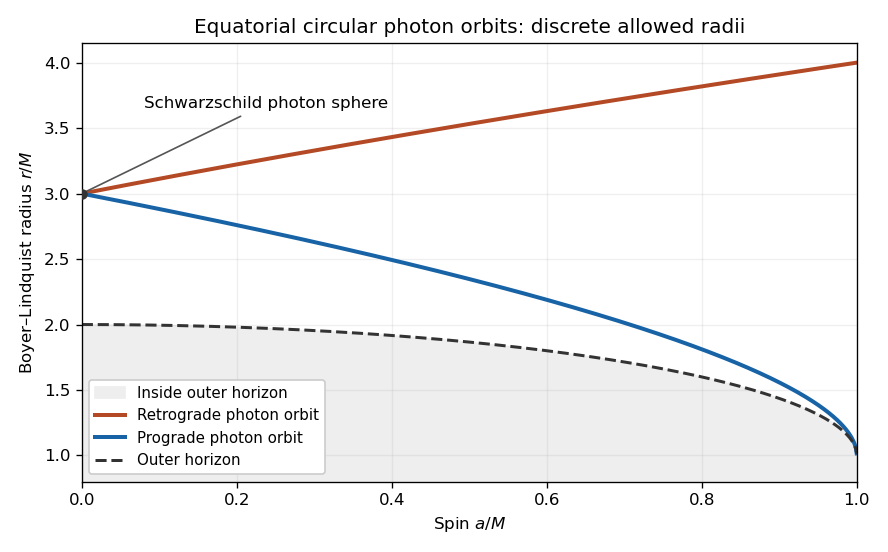
For a direct counterexample to the all-radii claim take and . Choose and so that . The radial geodesic equation nevertheless givesIt is a turning point, not a circular orbit. Alternatively, constant- null directions exist throughout the exterior because the two angular-velocity roots of are real; almost all of their integral curves require acceleration and fail the radial geodesic equation. This distinction explains how an all-radii assertion can arise.
Finally, itself has the null geodesic generators of its Killing horizon, proportional to . They are a separate horizon case. On the horizon is normal to every tangent, so its contractions with and both vanish: for a generator tangent. Its affine parameter can be chosen by rescaling that tangent. The exterior calculation dividing by does not include it. The presence of these generators does not supply circular null geodesics at the intervening arbitrary exterior radii.
Past exam of the general relativity II course of the University of Oxford 2017 3 c Solution by Codex 0 2026-10-25
Codex 0 2026-10-25Reflection across is an isometry; a geodesic initially tangent to its fixed equatorial plane remains in that plane by uniqueness of the geodesic equation. Thus take , , and . Define the algebraic abbreviationsThe conserved quantities of part (b) becomeFor , inversion givesThe null condition can be written without expanding a quadratic square:Substituting the preceding expressions yields the equatorial Kerr null geodesic radial equationAn equivalent useful polynomial form isThese expressions use an affine parameter ; a common rescaling of and accompanies its rescaling. The inversion was performed in the exterior , where Boyer-Lindquist coordinates are regular. The polynomial radial identity has a smooth continuation to a horizon, but the formulas for and there must be replaced by regular-coordinate expressions. In the limit , the result reduces to the Schwarzschild spacetime equation .
Past exam of the general relativity II course of the University of Oxford 2017 3 b Solution by Codex 0 2026-10-25
Codex 0 2026-10-25The metric tensor is independent of and , soare commuting Killing vector fields. For they span the continuous Killing vector field algebra; every constant linear combination is also a Killing vector field. They express stationary spacetime and axial symmetry, respectively. At the allowed endpoint the spherical symmetry of Schwarzschild spacetime enlarges the algebra: in addition to , a basis of rotational Killing vector fields isTheir polar-coordinate expressions are singular at the axis, but the rotational fields are smooth there.
Let be the tangent to any affinely parametrized geodesic. For a Killing vector field ,This is the geodesic conserved quantity from a Killing vector. With , choose the energy and axial angular momentum conventionsFor a massive particle with proper time parameter these are per unit rest mass; for a null geodesic their common scale depends on the affine parameter normalization. Expanding in the supplied Boyer-Lindquist coordinates givesThe factor of two between and the coefficient of is essential for these signs and coefficients.
Past exam of the general relativity II course of the University of Oxford 2017 3 a Solution by Codex 0 2026-10-25
Codex 0 2026-10-25A regular hypersurface , with , is a null hypersurface if its normal covector has zero squared norm:Its normal vector is then also tangent to the hypersurface; the induced metric tensor is degenerate.
For the Kerr metric the normal to a constant- surface has squared normFor the two roots are positive and distinct. To verify that they are genuine regular null hypersurfaces, rather than trusting singular Boyer-Lindquist coordinates, introduce ingoing Kerr coordinatesSubstitution givesThere are no terms. At either root , and the determinant is away from the angular coordinate poles. Thus the metric tensor extends smoothly across each root. The raised normal on either surface isThis is a nonzero null Killing vector field normal to the surface. Both surfaces are Killing horizons, with horizon angular velocities .
The event-horizon terminology in the paper needs qualification. In the usual asymptotically flat Kerr black hole extension, relative to a chosen exterior's future null infinity, the future branch of is the event horizon, the boundary . In the intervening black-hole region , the coordinate has timelike gradient and future-directed curves move toward smaller ; they cannot return across the outer boundary to that exterior. The inner surface is a Cauchy horizon, not a second event horizon for the same asymptotic end. Nullness is a local property; identifying an event horizon additionally requires this global causal structure.[ref]
General Relativity by David Tong. Sections 6.3.2 and 6.2.4: regular extension across the two Kerr roots, global diagram and the inner Cauchy horizon
The allowed endpoint provides an especially concrete counterexample to the unrestricted description of both roots. The Kerr metric then becomes Schwarzschild spacetime, is its regular event horizon, but is a curvature singularity:It is not a regular inner null hypersurface. Thus the two-horizon calculation above assumes .
Pinned article: Introduction to the OurBigBook Project
Welcome to the OurBigBook Project! Our goal is to create the perfect publishing platform for STEM subjects, and get university-level students to write the best free STEM tutorials ever.
Everyone is welcome to create an account and play with the site: ourbigbook.com/go/register. We belive that students themselves can write amazing tutorials, but teachers are welcome too. You can write about anything you want, it doesn't have to be STEM or even educational. Silly test content is very welcome and you won't be penalized in any way. Just keep it legal!
Intro to OurBigBook
. Source. We have two killer features:
- topics: topics group articles by different users with the same title, e.g. here is the topic for the "Fundamental Theorem of Calculus" ourbigbook.com/go/topic/fundamental-theorem-of-calculusArticles of different users are sorted by upvote within each article page. This feature is a bit like:
- a Wikipedia where each user can have their own version of each article
- a Q&A website like Stack Overflow, where multiple people can give their views on a given topic, and the best ones are sorted by upvote. Except you don't need to wait for someone to ask first, and any topic goes, no matter how narrow or broad
This feature makes it possible for readers to find better explanations of any topic created by other writers. And it allows writers to create an explanation in a place that readers might actually find it.
Figure 1. Screenshot of the "Derivative" topic page. View it live at: ourbigbook.com/go/topic/derivativeVideo 2. OurBigBook Web topics demo. Source. - local editing: you can store all your personal knowledge base content locally in a plaintext markup format that can be edited locally and published either:This way you can be sure that even if OurBigBook.com were to go down one day (which we have no plans to do as it is quite cheap to host!), your content will still be perfectly readable as a static site.
- to OurBigBook.com to get awesome multi-user features like topics and likes
- as HTML files to a static website, which you can host yourself for free on many external providers like GitHub Pages, and remain in full control

Figure 2. You can publish local OurBigBook lightweight markup files to either OurBigBook.com or as a static website.
Figure 3. Visual Studio Code extension installation.
Figure 5. . You can also edit articles on the Web editor without installing anything locally. Video 3. Edit locally and publish demo. Source. This shows editing OurBigBook Markup and publishing it using the Visual Studio Code extension. 
- Infinitely deep tables of contents:



All our software is open source and hosted at: github.com/ourbigbook/ourbigbook
Further documentation can be found at: docs.ourbigbook.com
Feel free to reach our to us for any help or suggestions: docs.ourbigbook.com/#contact