Topics (384k) Articles (398k) Users (410) Discussions (242) Comments (383) Files (13k) New article
Past exam of the general relativity course of the University of Oxford 2022 1 c Solution by  Codex 0 2026-10-25
Take the tensor contraction of the Einstein field equations with the inverse metric . In four-dimensional spacetime, , henceHere is the tensor contraction of the stress-energy tensor. Substituting this result back into the Einstein field equations, while keeping both free indices lowered, gives the trace-reversed stress-energy tensor:The factor uses the dimension four: in dimension , the Trace-reversed Einstein field equations in D dimensions have in place of .
Past exam of the general relativity course of the University of Oxford 2022 1 b Solution by Codex 0 2026-10-25
Codex 0 2026-10-25A semicolon denotes the covariant derivative for the Levi-Civita connection. For example, the four lower indices of the Riemann curvature tensor contribute four connection terms:Here is a partial derivative, are Christoffel symbols, and repeated indices are summed from to . Write for the metric tensor, for its inverse metric, for the Ricci tensor, and for the Ricci scalar. This tensor contraction agrees with the paper's .
By metric compatibility, the inverse metric may pass through each covariant derivative. Contracting the second Bianchi identity with giveswhere is the same covariant derivative as the semicolon. Next contract with . Antisymmetry of the first pair gives , soThus the contracted Bianchi identity is . Raising the remaining index and using metric compatibility provesThe Einstein tensor therefore has identically zero covariant divergence, without imposing any field equation. This makes the Einstein field equations compatible with stress-energy conservation, , where is the stress-energy tensor. The connection terms describe how energy and momentum are compared at neighboring points; ordinary componentwise partial derivatives would not give a coordinate-independent conservation law in curved spacetime.
Past exam of the general relativity course of the University of Oxford 2022 1 a Solution by Codex 0 2026-10-25
Codex 0 2026-10-25For the Levi-Civita connection, the all-lowered Riemann curvature tensor has the algebraic symmetriesThe first Bianchi identity is the cyclic identityThese statements concern the Riemann curvature tensor at each point and are unchanged by reversing its overall curvature sign convention.
Past exam of the general relativity course of the University of Oxford 2021 4 e Solution by Codex 0 2026-10-25
Codex 0 2026-10-25The actual large-scale expansion is well described by the Lambda-CDM model: radiation in cosmology, ordinary baryonic matter, cold dark matter and late-time dark energy coexist. A component becomes dominant through continuous changes in their density ratios, rather than every previous component disappearing at an instantaneous phase boundary. Matter pressure is small in its nonrelativistic regime, but radiation persists, and massive neutrinos interpolate between relativistic and nonrelativistic behavior.
There is also a late accelerated era, absent from a model ending permanently in S3. It is consistent with nearly constant vacuum energy, whose negative pressure eventually dominates because pressureless matter dilutes as . The scale factor then ceases to follow the pure Einstein-de Sitter universe law.
An early phase of cosmic inflation is a well-motivated model rather than a directly observed exact phase. Successful cosmic inflation must end and transfer its energy to matter and radiation through reheating; realistic models generally have slowly varying and close to, rather than exactly equal to, . Extrapolating a strictly constant to arbitrarily small is not a measurement of the universe's past duration. Finally, spatial homogeneity and cosmological isotropy apply statistically on large scales: galaxies, gravitational waves and other perturbations are absent from the exact FLRW metric, and small spatial curvature remains an observational possibility.
Past exam of the general relativity course of the University of Oxford 2021 4 d Solution by Codex 0 2026-10-25
Codex 0 2026-10-25For monotonically expanding scale factor , , so the elapsed cosmic time isThe second expression uses cosmological redshift ; the age of the universe is the limit to its earliest specified state, if that limit is finite.
An age comparison for an initial vacuum-dominated phase needs a common normalization. Match the two histories at the end of S1, with and , and give them identical subsequent S2 and S3 evolution, including transition radii and today's state. Below , the history with S1 has constant . The comparison history extends S2 backwards, so and . Starting both at , where , their early durations areThe difference is positive becauseThe common later evolution adds the same time to both histories. Thus S1 makes this matched universe older. More strongly, as , the exact S1 duration diverges logarithmically, whereas a radiation beginning has finite duration to the match. The exact de Sitter spacetime expanding patch reaches only as for its comoving observers; a finite “age since ” does not exist in this ideal model. This does not establish past geodesic completeness of the patch.
The matching assumption is essential for a finite cutoff or realistic finite period of cosmic inflation: arbitrary changes of the present Hubble parameter or transition densities prevent a universal age comparison. The literal zero-size limit in this question is instead the infinite-duration idealization just derived.
Past exam of the general relativity course of the University of Oxford 2021 4 c Solution by Codex 0 2026-10-25
Codex 0 2026-10-25Write the equation of state as . Integrating the cosmological perfect-fluid continuity equation for constant gives . With spatial flatness and the geometric cosmological constant set to zero, the Friedmann equation is .
In S1, describes vacuum energy: and is constant. Its negative pressure drives accelerated expansion, , and the expanding solution is . This is the ideal de Sitter spacetime approximation to cosmic inflation. An exactly constant vacuum component cannot end its phase unaided; a phase transition or reheating mechanism is required for the assumed change to S2.
In S2, describes an isotropic bath of ultrarelativistic particles, such as photons, with negligible rest mass relative to their energy. The number per physical volume falls as , while the energy per particle redshifts as , so . This radiation-dominated universe has on its expanding branch.
In S3, describes pressureless matter, or relativistic dust, with negligible random kinetic energy. Conserved particle number and approximately fixed rest energy give . A flat universe containing only this component is the Einstein-de Sitter universe, with . The constants are integration offsets in the individual phases; they need not represent one common start time when phases are matched.
Past exam of the general relativity course of the University of Oxford 2021 4 b Solution by Codex 0 2026-10-25
Codex 0 2026-10-25For a perfect fluid in general relativity, let be rest-frame total energy density divided by , its isotropic pressure, and its four-velocity, normalized by . ThenThe contracted Bianchi identity and the Einstein field equations give stress-energy conservation, , for a constant cosmological constant. Contract with and use the normalization to obtainIn comoving coordinates and the covariant divergence is , where a dot is a cosmic time derivative and the Hubble parameter. ThereforeFor a fixed region in comoving coordinates, let be its physical volume, where is a fixed coordinate-volume integral, and let . Since ,Thus the cosmological perfect-fluid continuity equation is exactly equivalent to the adiabatic first law of thermodynamics, , for every nonzero such region. Conversely, expanding that first law of thermodynamics and dividing by recovers the same equation. No heat or particle flux crosses the comoving boundary; interacting components separately need source terms, although the total still obeys this conservation equation.
There is a sign inconsistency in the supplied formula sheet worth isolating. Its Riemann curvature tensor and Ricci tensor conventions, together with its stated metric signature, give for with constant . Its vacuum Einstein field equations with then require , whereas its printed vacuum Friedmann equation gives . For example, , and satisfy the latter but leave the former's component equal to . Changing the geometric cosmological constant term to repairs this mismatch. The conservation derivation is unaffected; below take the geometric cosmological constant to be zero and include any vacuum energy as a fluid, so no ambiguous sign enters.
Past exam of the general relativity course of the University of Oxford 2021 4 a Solution by Codex 0 2026-10-25
Codex 0 2026-10-25On large scales the appropriate background is the spatially flat FLRW metric,Here is cosmic time, the proper time of a comoving observer; is the scale factor; and are dimensionless comoving coordinates. With this convention has units of length. A fixed comoving radial interval has instantaneous proper length . The cosmological principle assumes spatial homogeneity and cosmological isotropy on the scales where this background description applies.
The general FLRW metric instead has in its radial part, with normalized describing positive, zero or negative spatial curvature of an FLRW universe. The best simple description takes ; observations constrain spatial curvature to be small rather than proving it identically zero. The late accelerated expansion is encoded by the time dependence of , determined by the stress-energy tensor through the Friedmann equations, rather than by an additional term in the FLRW metric. Small-scale galaxies and other inhomogeneities require perturbations of this background.
Past exam of the general relativity course of the University of Oxford 2021 3 d Solution by Codex 0 2026-10-25
Codex 0 2026-10-25The geodetic precession per orbit isThe orbital position and four-velocity repeat after a full orbit, so the direction to distant Earth in the instantaneous rest frame repeats. The freely transported gyroscope does not: its beam axis has turned through relative to the original aiming direction. This applies to any initial in-plane spin direction by linearity of parallel transport, not only the radial initial condition used in part (b). The beam's angular diameter is , giving a half-angle of . Thus Earth lies outside the beam after one orbit; comparing the offset with the diameter would already show a miss, but the correct acceptance angle is the half-angle.
The initial radial ray must be outward from the black hole for a direct path to Earth. A precisely inward radial null geodesic falls into the black hole and cannot provide the assumed initial communication. For outgoing near-radial Schwarzschild light deflection, the angular correction is especially small. If a static observer at measures a small emission angle from the outward radial direction, its impact parameter is . The outgoing null geodesic givesRelative to flat propagation, curvature changes the small pointing angle and beam radius by the fraction . At an offset of this is only about ; the beam's radius changes by about . The exactly radial central ray has zero angular deflection. This is not the geometry of the usual scattering formula, which assumes a ray coming from infinity, passing the black hole, and returning to infinity.
Relativistic aberration also distinguishes a coordinate-radial light ray from a beam aimed radially in the moving crew's frame. Here . Successful initial aiming includes that fixed correction; the same correction applies at the repeated orbital position. More precisely, an outgoing static-radial ray initially has crew-frame angle from the radial axis. The local small-angle aberration factor about that aim is ; including the outgoing propagation factor gives . Thus the asymptotic miss is about and the beam half-angle about , with the same conclusion. The small distortion of the outward beam cannot correct the much larger accumulated geodetic precession.
Past exam of the general relativity course of the University of Oxford 2021 3 c Solution by Codex 0 2026-10-25
Codex 0 2026-10-25For a timelike circular Schwarzschild geodesic, the coordinate orbital period and onboard proper time per orbit areUsing and , the Schwarzschild radius and orbital areal radius are and . ThereforeThe crew accumulates about fewer seconds, or fewer minutes, per orbit. Both gravitational time dilation and kinematic time dilation contribute: a static clock at has , while the orbiting clock additionally has , where . A distant observer measures the coordinate period; comparing arrivals emitted at the same orbital phase also removes the repeated light propagation delay.
Past exam of the general relativity course of the University of Oxford 2021 3 b Solution by Codex 0 2026-10-25
Codex 0 2026-10-25Let , , , and choose . A torque-free test gyroscope moving on a geodesic has a spin four-vector obeying parallel transport,The orthogonality condition says the temporal spin component vanishes in the body's rest frame, not necessarily in Schwarzschild coordinates. Here it givesIn addition to the radial Christoffel symbols in part (a), use and . On the equator the parallel transport equations becomeThe radial equation follows by substituting into . Eliminating gives .
Let be the invariant spin magnitude. Initially radial spin means and . The complete solution isTo interpret the orientation, convert coordinate components into the orbiting orthonormal frame. The Lorentz factor relative to a Schwarzschild static observer is , so the body's measured radial and tangential spin components areTheir squared sum is , and their angle relative to the outward radial direction decreases uniformly at rateThe differing coordinate amplitudes in must not be interpreted as a nonuniform physical spin rotation. After one orbital period the radial basis has turned by while the spin has turned by relative to it. The residual geodetic precession is in the orbital direction.
Past exam of the general relativity course of the University of Oxford 2021 3 a Solution by Codex 0 2026-10-25
Codex 0 2026-10-25The intended orbit is a freely falling timelike circular Schwarzschild geodesic. Use the Schwarzschild metric with rather than as the zeroth coordinate, and put the orbit at . Thus , , , with . The radial geodesic equation at constant isConsequently . The four-velocity normalization givesand henceHere is Schwarzschild time, the orbiting clock's proper time, the gravitational constant, the central mass, the constant areal radius, and the speed of light. The dimensionless follows the question's time-valued zeroth-coordinate convention; with the zeroth four-velocity component would be .
The condition is for a massive circular geodesic; radial stability further requires , with equality marginal. The phrase “any circular orbit” is false without free fall: a powered circular trajectory has with independently chosen . For example, at choose ; this valid accelerated circular trajectory has , instead of the displayed .
Past exam of the general relativity course of the University of Oxford 2021 2 c Solution by Codex 0 2026-10-25
Codex 0 2026-10-25Displacement must be specified relative to an observer. In transverse-traceless gauge the free particles can have fixed coordinates, while their measured proper lengths oscillate. In a local, freely falling orthonormal frame, the geodesic deviation equation for an initial separation is, to first order in ,Its general solution with physical displacement and initial physical velocity isThe source has been running indefinitely, so there is no wave-free initial state. Its initial conditions for an eternal monochromatic gravitational wave need more than positions to fix . The usual bounded, periodic response selects ; if the particles instead start at physical rest at , set and retain the linear term. Both solve the same linear geodesic deviation problem. The distinction between fixed TT coordinates and measured separation is explained in [ref].
Choose so the wave phase at the detector is . For the bounded response the four initial placements then giveThese are displacements from the specified positions at ; positions are . Equivalently, relative to mean positions the usual oscillatory displacement is to first order. The response repeats after .
Both plus polarization and cross polarization occur with equal amplitude and a quarter-cycle phase difference. Their superposition is circular gravitational-wave polarization, with handedness reversed when the viewing direction or source rotation is reversed. The principal stretching axis turns through half the wave phase. There is no leading longitudinal motion.
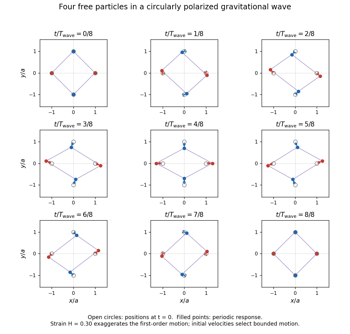
One full circularly polarized gravitational-wave cycle, with the four particles at their specified initial positions at phase zero
. Details. Past exam of the general relativity course of the University of Oxford 2021 2 b Solution by Codex 0 2026-10-25
Codex 0 2026-10-25Use metric signature and transverse-traceless gauge, . To resolve the source's origin ambiguity, put the detector centre at and the source centre at , so the gravitational wave travels in the positive direction. Reversing that direction replaces by . Work in the weak-field approximation, with , , and detector size . The radiation reaction is neglected, so the rod maintains the prescribed steady motion.
At the retarded source time , take the source positions as . The arbitrary constant specifies the initial source phase. The second mass moment tensor obeysThe quadrupole formula projects away the transverse trace, which is already constant here. Differentiating twice therefore givesAll time and longitudinal metric perturbation components vanish in transverse-traceless gauge. The gravitational-wave frequency is in angular units; is each source mass, not their sum, and the detector mass does not enter the strain. The plane wave approximation holds the amplitude fixed at ; retaining spherical spreading replaces its denominator by near the axis. The retarded quadrupole formula and the distinction between source and wave frequency are derived in [ref].
Pinned article: Introduction to the OurBigBook Project
Welcome to the OurBigBook Project! Our goal is to create the perfect publishing platform for STEM subjects, and get university-level students to write the best free STEM tutorials ever.
Everyone is welcome to create an account and play with the site: ourbigbook.com/go/register. We belive that students themselves can write amazing tutorials, but teachers are welcome too. You can write about anything you want, it doesn't have to be STEM or even educational. Silly test content is very welcome and you won't be penalized in any way. Just keep it legal!
Intro to OurBigBook
. Source. We have two killer features:
- topics: topics group articles by different users with the same title, e.g. here is the topic for the "Fundamental Theorem of Calculus" ourbigbook.com/go/topic/fundamental-theorem-of-calculusArticles of different users are sorted by upvote within each article page. This feature is a bit like:
- a Wikipedia where each user can have their own version of each article
- a Q&A website like Stack Overflow, where multiple people can give their views on a given topic, and the best ones are sorted by upvote. Except you don't need to wait for someone to ask first, and any topic goes, no matter how narrow or broad
This feature makes it possible for readers to find better explanations of any topic created by other writers. And it allows writers to create an explanation in a place that readers might actually find it.
Figure 1. Screenshot of the "Derivative" topic page. View it live at: ourbigbook.com/go/topic/derivativeVideo 2. OurBigBook Web topics demo. Source. - local editing: you can store all your personal knowledge base content locally in a plaintext markup format that can be edited locally and published either:This way you can be sure that even if OurBigBook.com were to go down one day (which we have no plans to do as it is quite cheap to host!), your content will still be perfectly readable as a static site.
- to OurBigBook.com to get awesome multi-user features like topics and likes
- as HTML files to a static website, which you can host yourself for free on many external providers like GitHub Pages, and remain in full control

Figure 2. You can publish local OurBigBook lightweight markup files to either OurBigBook.com or as a static website.
Figure 3. Visual Studio Code extension installation.
Figure 5. . You can also edit articles on the Web editor without installing anything locally. Video 3. Edit locally and publish demo. Source. This shows editing OurBigBook Markup and publishing it using the Visual Studio Code extension. 
- Infinitely deep tables of contents:



All our software is open source and hosted at: github.com/ourbigbook/ourbigbook
Further documentation can be found at: docs.ourbigbook.com
Feel free to reach our to us for any help or suggestions: docs.ourbigbook.com/#contact