Topics (384k) Articles (398k) Users (410) Discussions (242) Comments (383) Files (13k) New article
Past exam of the geophysical fluid dynamics course of the University of Oxford 2023 1 c Solution by  Codex 0 2026-10-25
Take eastward , upward , positive wavenumbers , and a real instantaneous amplitude . A common growing factor does not affect the phase geometry. Put and , using the hyperbolic cosine and hyperbolic sine. The prescribed streamfunction iswhereFollowing a fixed phase givesTherefore the streamfunction pattern tilts westward with height. The lower boundary leads the upper boundary eastward.
In the conventional quasi-geostrophic streamfunction normalization, hydrostatic balance gives . ThereforeFor the phase calculation, multiplication by the constant is immaterial. Define a continuous phase ; this avoids a spurious discontinuity at . ThenThe buoyancy perturbation pattern tilts eastward with height, opposite to the streamfunction pattern. At , while , so the two fields are a quarter wavelength apart there.
Both perturbation amplitudes are largest at the boundaries. Indeed,which increase with . The physical reason is particularly clear through stratified quasi-geostrophic inversion: the Eady model has no interior background potential-vorticity gradient, and a growing normal mode has zero interior potential vorticity anomaly. The independent thermal anomalies reside at the rigid upper and lower boundaries, where meridional motion advects the basic horizontal buoyancy gradient. Each Eady edge wave induces an interior balanced flow that decays away from its boundary on scale . Their interacting, phase-locked combination produces the growing baroclinic instability. Boundary confinement of the thermal sources, rather than a rigid-wall requirement , explains the amplitude pattern.
For a sketch with a quarter-wavelength difference between the boundary streamfunction patterns, chooseAn upper positive streamfunction crest is then west of its lower counterpart, where . The buoyancy perturbation crests slope the other way. The quarter-wavelength boundary assumption is used for the streamfunction; differentiating in fixes the buoyancy perturbation and does not generally give it the same boundary phase separation.
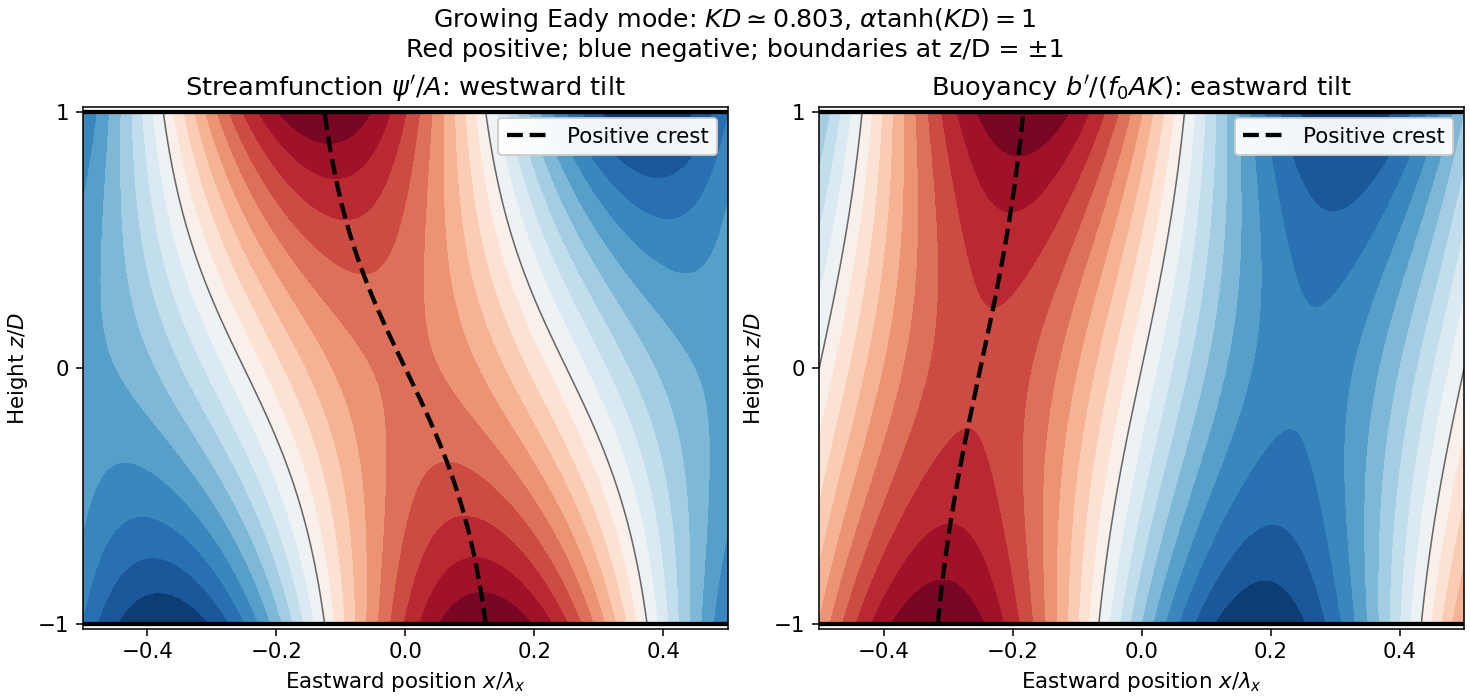
Original Eady model sketch: streamfunction crests tilt westward and buoyancy perturbation crests eastward. Dashed curves follow positive maxima; the streamfunction boundary phase difference is a quarter wavelength.
Details. The connection to poleward heat transport can be checked without relying on the sketch. The meridional geostrophic flow and buoyancy perturbation areAverage over one zonal wavelength, using equal averages for squared sine and cosine and zero for their product:In the Northern Hemisphere this is positive: warm anomalies preferentially move northward and cold anomalies southward. For the same eastward-increasing basic thermal wind in the Southern Hemisphere, and the basic buoyancy gradient reverses; the negative northward eddy buoyancy flux is again poleward. For thermal expansion coefficient and specific heat capacity at constant pressure , the corresponding sensible heat flux in a thermal Boussinesq approximation is . The growing amplitude makes this flux grow as . The tilt supplies the correlation absent in an untilted disturbance and reduces the background available potential energy.
Past exam of the geophysical fluid dynamics course of the University of Oxford 2023 1 b Solution by Codex 0 2026-10-25
Codex 0 2026-10-25Let denote the actual horizontal velocity field. With constant nonzero Coriolis parameter , geostrophic balance and hydrostatic balance, using pressure per reference density , giveDifferentiate the first equation in to obtain thermal-wind balance:Taking the dot product with provesThus the horizontal velocity is tangent to the horizontal buoyancy contours at every height. For a fluid whose thermal equation of state makes horizontal buoyancy contours coincide with horizontal temperature contours, there is no horizontal advection across those contours. In a dry terrestrial atmosphere, use potential temperature as the materially conserved thermal variable. A salinity contribution to buoyancy would require separate treatment before interpreting the result as a statement about temperature.
The usual statement about net meridional heat transport also follows explicitly. Introduce a horizontal streamfunction such that . Integration of thermal-wind balance givesand henceFor a zonally periodic function , or vanishing endpoint contributions, the zonal integral is zero. Likewise, the anomalous eddy buoyancy flux isThe required correlation between meridional velocity and thermal anomaly is absent. A nonzero vertical phase tilt, as in the next part, permits that correlation.
Qualification of the wording. The result does not say that the local heat flux vector vanishes, or that an arbitrary open-domain integral vanishes without boundary conditions. For a concrete counterexample to that literal reading, take and . These satisfy the displayed thermal-wind balance, but is generally nonzero. What the hypotheses alone guarantee is zero transport across horizontal buoyancy contours; the vanishing zonally integrated heat transport uses the stated endpoint condition.
Past exam of the geophysical fluid dynamics course of the University of Oxford 2023 1 a Solution by Codex 0 2026-10-25
Codex 0 2026-10-25Choose northward and upward in the Northern Hemisphere. In a locally linear Boussinesq approximation, write the background buoyancy as , with horizontal buoyancy gradient and positive squared buoyancy frequency . The stable density stratification resists a purely vertical displacement, but the isopycnals slope upward poleward:The geopotential surfaces are horizontal in this local approximation. Their inclination differs from that of the isopycnals, which is the relevant baroclinicity.
Exchange two equal small fluid elements, each of volume , between positions separated by . The adiabatic parcel exchange has no thermal diffusion, so each parcel retains its buoyancy. The background buoyancy difference is . Because the variable-density contribution to gravitational potential energy is , the change in the pair's gravitational potential energy isFor a poleward-rising exchange, set with . ThenThe trajectory lies between a geopotential surface and an isopycnal. The poleward-rising parcel starts more buoyant than the parcel it replaces, and the equatorward-sinking parcel starts less buoyant: the buoyancy does positive work on both. This releases available potential energy into kinetic energy, allowing eddies to amplify if the full rotating dynamics supports the displacement and dissipation does not remove the gain.
A trajectory steeper than the isopycnals, , instead costs gravitational potential energy; an equatorward-rising trajectory also costs it. Motion exactly along a geopotential surface or an isopycnal gives zero change in this ideal exchange. At fixed , the largest release occurs at , since is minimized there.
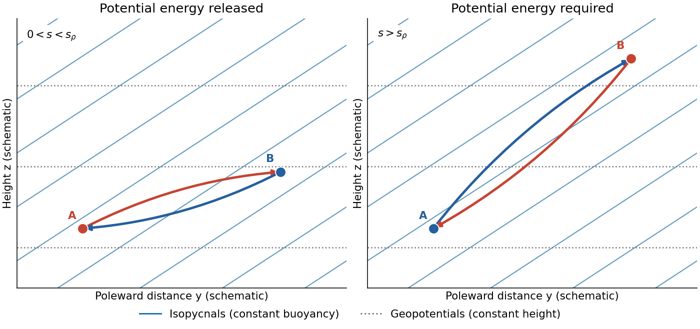
Two adiabatic parcel exchanges: a shallow poleward rise releases potential energy, whereas a rise steeper than the isopycnals costs it. Slopes are exaggerated.
Details. This is an energetic possibility argument for baroclinic instability, not a sufficient normal mode instability criterion. In particular, unrestricted parcel motion must not be assumed in a rotating fluid: conservation of angular momentum can impose an additional restoring effect. Symmetric instability has a separate Ertel potential vorticity criterion; ordinary Eady instability can occur without violating that criterion.
Past exam of the geometry of surfaces course of the University of Oxford 2023 3 f Solution by Codex 0 2026-10-25
Codex 0 2026-10-25For , let and use the orientation of a surface determined by . Its positive boundary orientation follows the bottom side in increasing , the right side in increasing , the top side in decreasing , and the left side in decreasing . The Gauss-Bonnet theorem for this disc with four corners readswhere the are the signed exterior angles.
The bottom and top sides have cancelling geodesic curvature integrals: a screw motion takes one to the other with opposite boundary orientation. Explicitly, along increasing at fixed , the speed is one and the signed geodesic curvature is on both sides. The right and left sides contribute, respectively, the integral along and minus the integral along .
Although the coordinate sides are generally not perpendicular, the corner contributions still sum to . Indeed, let be the angle between and , soStarting at the bottom-left corner, the exterior angles are , , and . Their sum is . Cancelling this from the Gauss-Bonnet theorem leaveswhich is the identity in part (e). For a rectangle covering more than one turn, apply the same argument on the parameter rectangle with its induced Riemannian metric, or partition it into narrower rectangles and cancel the artificial internal boundary contributions. This gives the version counting multiplicity, as required by the correction in part (e).
Past exam of the geometry of surfaces course of the University of Oxford 2023 3 e Solution by Codex 0 2026-10-25
Codex 0 2026-10-25First interpret the surface integral through the given parametric surface, counting multiplicity. SetIts derivative isUsing part (c), the fundamental theorem of calculus givesOn the other hand part (d), including its arc length factor, givesand the corresponding expression for is . Subtraction provesIf , the parametric surface is injective on the rectangle, so this is exactly the stated surface integral over its image. It also remains the ordinary image integral at , since the repeated seam has zero surface area.
The assertion for arbitrary needs a multiplicity convention or the restriction . This omission is present in the native PDF. For example, take , , , . The image is the entire cylindrical band , since already covers a full turn. Its ordinary surface integral of Gaussian curvature isBut the difference of the two signed geodesic curvature integrals is . Thus ordinary integration over the image set makes the unrestricted assertion false. The boxed parameter integral is valid for all and and is the appropriate corrected statement. This distinction is the multiplicity of a parametrized surface integral.
Past exam of the geometry of surfaces course of the University of Oxford 2023 3 d Solution by Codex 0 2026-10-25
Codex 0 2026-10-25Use the unit normal from part (c), and orient by increasing . Write for its unit tangent vector. The signed geodesic curvature convention used below iswhere is arc length. The second equality follows by differentiating : the term parallel to disappears in the scalar triple product. It makes the correction for a parameter which is not arc-length parametrization explicit.
Put , , , and . The speed is the constant . At ,soTaking its dot product with yields . ThereforeThe screw motion of part (b) makes this independent of . Thus is a geodesic precisely when is an integer multiple of . Reversing the direction of traversal or the unit normal changes the sign of signed geodesic curvature; its magnitude is the absolute value of the displayed expression. The signed convention is needed in part (e).
Past exam of the geometry of surfaces course of the University of Oxford 2023 3 c Solution by Codex 0 2026-10-25
Codex 0 2026-10-25Set , , and . At , the first partial derivatives areTheir dot products give , , . HenceSince , the parametric surface is regular everywhere. Its cross product and unit normal at areThe second partial derivatives at areTheir dot products with give and . ThusPart (b) transports these first fundamental form and second fundamental form coefficients to every . Finally,The last expression is the surface area element from . In particular the Gaussian curvature changes sign where does; it vanishes at modulo .
Past exam of the geometry of surfaces course of the University of Oxford 2023 3 b Solution by Codex 0 2026-10-25
Codex 0 2026-10-25Let be the horizontal rotation matrix through angle . Define the screw motionIts linear part is an orthogonal matrix with determinant one, and its remaining part is a translation. Thus it is a proper Euclidean motion of Euclidean three-space, with .
In horizontal-vector notation the given parametric surface satisfies . ThereforeThe defining circle in each horizontal plane is entirely parametrized by , so covers . The displayed equality and prove . This one-parameter subgroup preserves the dot products and cross products defining , and the chosen unit normal. Consequently their coordinate coefficients, and the Gaussian curvature, depend only on .
Past exam of the geometry of surfaces course of the University of Oxford 2023 3 a Solution by Codex 0 2026-10-25
Codex 0 2026-10-25For a regular parametric surface , its tangent vectors are linearly independent. The first fundamental form is the induced inner product on the tangent plane, writtenIt measures squared lengths and angles; its determinant satisfies . Choose the unit normalThe second fundamental form, with shape operator , isThe subscript distinguishes the coefficient from a genus or a Riemannian metric. In these coordinates the shape operator has matrix , so the Gaussian curvature, the product of its two principal curvatures, isReversing reverses and both principal curvatures, leaving the Gaussian curvature unchanged.
Past exam of the geometry of surfaces course of the University of Oxford 2023 2 e Solution by Codex 0 2026-10-25
Codex 0 2026-10-25The dihedral group here has order . Substituting into part (d) givesIn particular, requires genus seven. A geometric construction is to start with a round solid torus about the vertical axis, then drill thin radial tunnels through its tube in the horizontal midplane, equally spaced at azimuths , . The tunnels run from the central opening to the exterior; their directions are horizontal and radial. Round all their rims in the same way, preserving the dihedral symmetry, and let be the boundary of the resulting solid.
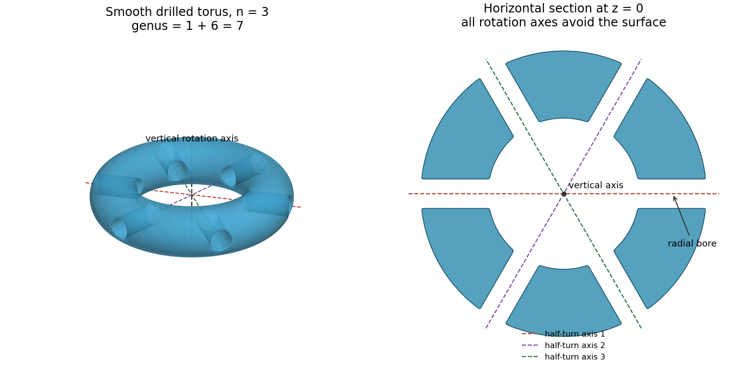
A genus-seven surface with a free dihedral action: six radial bores contain the horizontal rotation axes
. Details. Here is why the construction has exactly the required properties. Every nonidentity power of is a rotation in three dimensions fixing the vertical axis, which lies in the central opening and is disjoint from . Each element is a half-turn about a horizontal line at azimuth , modulo . The such lines meet the original solid torus in short radial segments. Each segment lies strictly inside one drilled tunnel, so these axes are also disjoint from . A nonidentity rotation in three dimensions fixes only its axis. Thus no nonidentity element fixes a point of , proving a free action of a group.
Rotation by permutes the tunnels, while preserves their arrangement and the original solid torus. Hence is preserved by the two generators and therefore by . The tunnels can be chosen sufficiently thin to be pairwise disjoint, and the rounding can be made group-invariant in small disjoint neighbourhoods of their rims. It neither changes the genus nor introduces an intersection with any axis.
Each tunnel removes two discs from the existing boundary and inserts the cylindrical wall of the bore. Its contribution to Euler characteristic is : the two removed discs contribute , and the inserted annulus and its boundary circles have zero Euler characteristic. The boundary remains connected and orientable, so each tunnel increases genus by one. Starting from a torus and drilling tunnels therefore gives . The construction also supplies a Riemann surface: use the complex structure associated with the induced oriented Riemannian metric. The ambient generators are isometries preserving the solid and ambient orientation of a vector space, so they preserve the induced boundary orientation and act by biholomorphisms. Part (d) then confirms that the quotient space has genus two. This is a free dihedral action on a drilled torus.
Past exam of the geometry of surfaces course of the University of Oxford 2023 2 d Solution by Codex 0 2026-10-25
Codex 0 2026-10-25For a free action of a group, every stabilizer subgroup is trivial. Hence every ramification index of a holomorphic map is one, and the projection is an unramified covering map of degree of a holomorphic map . The Riemann-Hurwitz formula reduces toThis is also the multiplicativity of Euler characteristic under a finite covering.
Past exam of the geometry of surfaces course of the University of Oxford 2023 2 c Solution by Codex 0 2026-10-25
Codex 0 2026-10-25In a cyclic group of prime order , a stabilizer subgroup has order either one or . The latter case consists exactly of points fixed by all of . Thus the fixed points each have ramification index of a holomorphic map , and every other point has index one. Applying the Riemann-Hurwitz formula with degree of a holomorphic map givesEquivalently,The count concerns fixed points upstairs. Each is its own group orbit, so their images are also distinct branch values of a holomorphic map.
Past exam of the geometry of surfaces course of the University of Oxford 2023 2 b Solution by Codex 0 2026-10-25
Codex 0 2026-10-25Every nonidentity biholomorphism in the finite group has only finitely many fixed points, by the identity theorem on a Riemann surface and compactness. Because the group action is a faithful group action, the union of these finite sets does not exhaust . A point outside this union has trivial stabilizer subgroup, so its group orbit has points by the orbit-stabilizer theorem. The generic fiber of a function of the projection is such an group orbit, givingMore precisely, put and . Differentiation at gives a group homomorphism . It is injective: if a nonidentity finite-order germ had the form with and , then its th iterate would begin , so no positive iterate could be the identity. A germ equal to the identity gives the identity on by the identity theorem on a Riemann surface. Thus is a cyclic group, with derivative image the th roots of unity.
For completeness, an explicit local coordinate linearizing isIt has , and reindexing the sum gives . Therefore a coordinate on the local quotient space is . Other translates of a sufficiently small neighbourhood of are disjoint unless their translating element lies in , so this local quotient space is also a chart for . The local cyclic quotient of a Riemann surface consequently gives
Past exam of the geometry of surfaces course of the University of Oxford 2023 2 a Solution by Codex 0 2026-10-25
Codex 0 2026-10-25Let and choose holomorphic coordinate charts centred at and . A nonconstant holomorphic map has a local expansion , where and . Taking a local holomorphic th root of the nonvanishing factor and changing the source coordinate gives the exact local form . The integeris the ramification index of a holomorphic map. A ramification point of a holomorphic map is a source point with , equivalently where its derivative vanishes; a branch value of a holomorphic map, also called a branch point here, is the image of such a point in . These are different sets, one in the source and one in the target.
Every fiber of a function is finite: locally it is the zero set of a nonzero holomorphic function, so its points are isolated, and compactness prevents infinitely many such zeros without an accumulation point. The same argument applied to the local derivatives makes the set of ramification points of a holomorphic map finite. The open mapping theorem and compactness show that is both open and closed in the connected target , hence is surjective.
For any , the degree of a holomorphic map isTo see independence of , choose disjoint small coordinate charts about its finitely many preimages. The local form shows that nearby values have preimages counted with multiplicity in the corresponding chart. Compactness excludes additional preimages outside these charts for sufficiently nearby values: a sequence of such preimages would have a limit in . The displayed sum is therefore locally constant, hence constant on connected . Away from branch values of a holomorphic map it is the ordinary number of preimages, and is a -sheeted covering map there.
The Riemann-Hurwitz formula isor, in terms of the two genera,For its proof, choose a triangulation of a surface on containing every branch value of a holomorphic map among its vertices. Every open edge and open face has lifts, since its interior avoids branch values of a holomorphic map. The lifted cells give a finite CW complex structure on . If are the target counts and , the source counts areIndeed, at a target vertex the deficit from distinct preimages is precisely , and all nonzero contributions occur over vertices. Taking the alternating sum gives , as required. This is the Triangulation proof of the Riemann-Hurwitz formula.
Past exam of the geometry of surfaces course of the University of Oxford 2023 1 e Solution by Codex 0 2026-10-25
Codex 0 2026-10-25Take a hexagonal polygonal schema with boundary wordIdentify equally labelled polygon edges in the indicated directions. The two consecutive occurrences of identify the first three vertices; the two edges extend this class to the next two vertices, and the edges include the remaining vertex. Thus all six polygon vertices become one, while the six edges become three and the interior is one face. Its Euler characteristic isThis is the usual polygonal schema for the connected sum of surfaces of three real projective planes. The same-sign edge pairs force a nonorientable surface, consistently with . A closed orientable surface cannot have odd Euler characteristic.
Past exam of the geometry of surfaces course of the University of Oxford 2023 1 d Solution by Codex 0 2026-10-25
Codex 0 2026-10-25The uniformization theorem says that every simply connected Riemann surface is biholomorphic to the Riemann sphere, the complex plane, or the unit disc. Its consequence for a compact Riemann surface of genus at least two is that the universal cover is the unit disc, equivalently the hyperbolic plane.
To explain the restriction, a spherical universal cover would make the fundamental group finite. Since a finite covering map multiplies Euler characteristic, is impossible for . If the universal cover were the complex plane, its deck transformations would be biholomorphisms . A nonidentity such map with has a fixed point, impossible for a deck transformation. Thus the deck transformation group would consist of translations. A discrete subgroup of translations with compact quotient space is a rank-two Euclidean lattice, whose quotient space is a torus, again incompatible with .
On the unit disc, the Poincare metric on a Riemann surfacehas Gaussian curvature and is invariant under every biholomorphism of the unit disc. It therefore descends through the deck transformation group to a hyperbolic metric on . Its local expression is a positive multiple of in every holomorphic coordinate chart, so it is compatible with the given complex structure. In fact, this hyperbolic metric is unique within that conformal class.
Past exam of the geometry of surfaces course of the University of Oxford 2023 1 c Solution by Codex 0 2026-10-25
Codex 0 2026-10-25Write for the internal angle at , using the numbering in part (b), and use the hyperbolic plane with Gaussian curvature . The necessary and sufficient conditions are equal lengths for each pair of equally labelled polygon sides, and total angle at each vertex equivalence class. Explicitly, the two angle conditions areNecessity follows because the identification must preserve arc length along each seam, and a smooth interior point of a Riemannian surface has total angle . For sufficiency, equally long hyperbolic geodesic segments can be identified by isometries. Across their interiors, two half-disc neighbourhoods join to a hyperbolic disc. At an identified vertex, the incident sectors form a cyclic disc with total angle , so no cone singularity of a surface metric remains. These local isometries therefore extend the Riemannian metric smoothly everywhere. This is the smooth hyperbolic polygon gluing criterion.
The ten internal angles sum to . The area of a hyperbolic geodesic polygon consequently givesEquivalently, the Gauss-Bonnet theorem gives .
Past exam of the geometry of surfaces course of the University of Oxford 2023 1 b Solution by Codex 0 2026-10-25
Codex 0 2026-10-25Number the polygon vertices in the order of the given polygonal schema, with its th polygon edge going from to , and subscripts interpreted modulo ten. Equal labels identify equal arrow endpoints. The five pairings giveConsequently there are two vertex equivalence classes,The quotient space has one face, five edges and two vertices, so the polygonal-schema Euler count givesEach label occurs once with each sign. Hence every pairing reverses the direction induced by traversing the boundary of the polygon, so an orientation of a surface on its interior extends consistently across every glued edge. Thus is orientable. The classification of compact surfaces now gives , or a closed orientable surface of genus two, equivalently the connected sum of surfaces of two tori.
Past exam of the geometry of surfaces course of the University of Oxford 2023 1 a Solution by Codex 0 2026-10-25
Codex 0 2026-10-25The classification of compact surfaces says that every compact, connected topological surface without boundary is homeomorphic to exactly one of the following: the sphere ; a connected sum of surfaces consisting of tori; or a connected sum of surfaces consisting of real projective planes. The first two cases are orientable; the last case is a nonorientable surface. Their Euler characteristics areHere has genus , and has crosscaps; is the real projective plane and the Klein bottle. Thus orientability together with the Euler characteristic determines the closed surface up to homeomorphism.
If the convention permits a surface with boundary, also remove the interiors of disjoint closed discs from one of these closed surfaces. The Euler characteristic decreases by , giving in the orientable case and in the nonorientable surface case. The number of boundary components is then an additional invariant.
Past exam of the general relativity II course of the University of Oxford 2021 3 c Solution by Codex 0 2026-10-25
Codex 0 2026-10-25First use the original null coordinates , . They obey , and the radial metric tensor becomesApply the given substitutions and . The identitiesgive the analytic extension of a spacetimeThe poles of the individual tangent and cotangent substitutions are now ordinary coordinate lines wherever . Set and . Allowing these coordinate functions to continue across every such line givesThis is the universal cover of two-dimensional anti-de Sitter spacetime of radius , times a two-sphere of radius : the simply connected Bertotti-Robinson spacetime. In defining this maximal analytic extension, ranges over the whole real line without periodic identification. A periodic identification would instead create closed timelike curves and would be an additional global choice.
For clarity, the original patch is embedded by the branches and . The inequality is equivalent on these branches to , so the original patch occupiesThe first spacetime extension in part (a) occupies the larger band , with . Its finite- Killing horizon is the interior line . The edges of that band are further regular Poincaré horizons; continuing through them produces the full conformal strip of two-dimensional anti-de Sitter spacetime.
The original coordinate has a smooth continuation throughout the strip:Consequently the complete set of zero-level Killing horizons isThese are two alternating families of parallel null lines; different families meet only at the excluded conformal boundaries, never inside the spacetime. The continuation of the original Killing vector field isThe field never vanishes in the interior, including on the Killing horizons.
To obtain the Penrose diagram, suppress the two-sphere and multiply by the conformal factor . The resulting radial metric tensor is , so the diagram is an infinitely tall strip of width , with null lines at 45 degrees and timelike edges . Generically,At the special edge points where the two families of Killing horizons end, the displayed formula is a limit and has no unique limiting value. Thus the infinity labels on the diagram refer to the open edge segments, not those vertices. Each interior point of the diagram represents a two-sphere of fixed radius ; neither edge is a centre where that two-sphere shrinks.
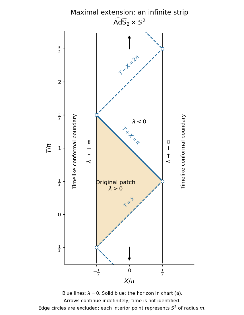
Penrose diagram of the maximal Bertotti-Robinson spacetime extension, with the original patch and all zero-level Killing horizons
. Details. Finally, these timelike edges are conformal boundaries, not omitted regular points of a further spacetime extension. One way to establish maximality is geodesic completeness. The two-dimensional anti-de Sitter spacetime factor embeds locally as in a flat space with metric signature . Along an affinely parametrized geodesic with constant , the ambient equation isIts oscillatory, linear or hyperbolic solutions for negative, zero or positive exist for all real affine parameters and lift to the universal cover. The two-sphere is also geodesically complete, and geodesics of the product split into geodesics of its factors. Hence is geodesically complete. A proper regular spacetime extension would furnish a geodesic reaching its boundary in finite affine parameter, contradicting that completeness. This proves that the displayed simply connected analytic spacetime is maximal.
Pinned article: Introduction to the OurBigBook Project
Welcome to the OurBigBook Project! Our goal is to create the perfect publishing platform for STEM subjects, and get university-level students to write the best free STEM tutorials ever.
Everyone is welcome to create an account and play with the site: ourbigbook.com/go/register. We belive that students themselves can write amazing tutorials, but teachers are welcome too. You can write about anything you want, it doesn't have to be STEM or even educational. Silly test content is very welcome and you won't be penalized in any way. Just keep it legal!
Intro to OurBigBook
. Source. We have two killer features:
- topics: topics group articles by different users with the same title, e.g. here is the topic for the "Fundamental Theorem of Calculus" ourbigbook.com/go/topic/fundamental-theorem-of-calculusArticles of different users are sorted by upvote within each article page. This feature is a bit like:
- a Wikipedia where each user can have their own version of each article
- a Q&A website like Stack Overflow, where multiple people can give their views on a given topic, and the best ones are sorted by upvote. Except you don't need to wait for someone to ask first, and any topic goes, no matter how narrow or broad
This feature makes it possible for readers to find better explanations of any topic created by other writers. And it allows writers to create an explanation in a place that readers might actually find it.
Figure 1. Screenshot of the "Derivative" topic page. View it live at: ourbigbook.com/go/topic/derivativeVideo 2. OurBigBook Web topics demo. Source. - local editing: you can store all your personal knowledge base content locally in a plaintext markup format that can be edited locally and published either:This way you can be sure that even if OurBigBook.com were to go down one day (which we have no plans to do as it is quite cheap to host!), your content will still be perfectly readable as a static site.
- to OurBigBook.com to get awesome multi-user features like topics and likes
- as HTML files to a static website, which you can host yourself for free on many external providers like GitHub Pages, and remain in full control

Figure 2. You can publish local OurBigBook lightweight markup files to either OurBigBook.com or as a static website.
Figure 3. Visual Studio Code extension installation.
Figure 5. . You can also edit articles on the Web editor without installing anything locally. Video 3. Edit locally and publish demo. Source. This shows editing OurBigBook Markup and publishing it using the Visual Studio Code extension. 
- Infinitely deep tables of contents:




All our software is open source and hosted at: github.com/ourbigbook/ourbigbook
Further documentation can be found at: docs.ourbigbook.com
Feel free to reach our to us for any help or suggestions: docs.ourbigbook.com/#contact