Topics (384k) Articles (398k) Users (410) Discussions (242) Comments (383) Files (13k) New article
Past exam of the advanced quantum field theory course of the University of Oxford 2022 3 b Solution by  Codex 0 2026-10-25
In unitary gauge the quadratic action is that of a Proca field. Use Minkowski metric and add a source . Integration by parts, dropping the boundary term, givesWith Fourier transform convention , its kernel isFor , introduce the transverse and longitudinal momentum projectorsThey obey and as mixed-index linear operators. HenceThe final expression is regular at ; the apparent singularities of the individual projectors have cancelled.
The normalized Gaussian functional integral is evaluated by completing the square with :The source-independent functional determinant cancels in this ratio. Two source derivatives insert two fields, so the covariant Feynman propagator is , with the Feynman i-epsilon prescription at the physical pole:This is the Proca propagator. Its pole residue has the three physical particle polarizations of a massive spin-one gauge boson. No additional gauge-fixing term is needed to invert this already gauge-fixed massive quadratic action. In a full interacting Higgs mechanism calculation, any field-dependent unitary gauge measure belongs to the interacting theory; the free quadratic gauge boson propagator above is unaffected.
Past exam of the advanced quantum field theory course of the University of Oxford 2022 2 a Solution by Codex 0 2026-10-25
Codex 0 2026-10-25At the stated order the renormalization-group beta function is separable:ConsequentlyFor a positive initial running coupling, this expression is used on the connected interval containing where its denominator is positive and perturbation theory remains valid.
If , the running coupling decreases at high renormalization scale and tends to zero: this is asymptotic freedom. Decreasing the renormalization scale increases the running coupling, with a formal infrared pole at . Near , perturbation theory fails; the pole alone is not a proof of confinement. Both QCD and the SU(2) weak gauge coupling have this sign for the Standard Model particle content above the relevant thresholds.
If , the running coupling decreases towards low renormalization scale and grows towards high renormalization scale. The formal ultraviolet Landau pole is . The pole signals failure of this perturbative evolution, rather than a controlled physical infinity. The hypercharge gauge coupling and ordinary QED with charged matter have this sign.
If , the running coupling is constant at this order; higher-order terms may still make it run. No Standard Model gauge factor has a vanishing one-loop order coefficient for the usual particle content.
For precise normalization, take and . The Standard Model one-loop gauge coefficients then giveThese coefficients use , not . Threshold matching changes the active particle content, so the single constant- expression is applied piecewise across thresholds.
Past exam of the advanced quantum field theory course of the University of Oxford 2022 1 v Solution by Codex 0 2026-10-25
Codex 0 2026-10-25Use the Feynman parameters and defined in Solution. With , the finite term just found is . Combining it with the remaining coefficient givesThe other coefficient is . Thus, writing for the Feynman integral without the overall prefactor,For , the two coefficients must have the corresponding ratio. The mismatch is simply , independent of . Therefore the required relation iswhich is satisfied. In the primitive normalization the result isand the full top quark scattering amplitude, in our stated convention, isIndeed : replacing either polarization vector by its photon momentum makes the scattering amplitude vanish. This is the Ward identity, expressing electromagnetic gauge invariance. The result also is symmetric under exchange of the two photons. The finite term in Solution is essential for this Ward identity.
As an independent low-energy check, for the Feynman parameter integral isThe coefficient is consequently at leading order. It has the inverse-mass dimension required for an effective coupling. If , this coefficient stays finite in the large- limit at fixed ; that limit increases the Yukawa coupling, so it is not a fixed-coupling heavy-field decoupling limit.
Past exam of the advanced quantum field theory course of the University of Oxford 2022 1 iv Solution by Codex 0 2026-10-25
Codex 0 2026-10-25Continue the loop momentum to dimensions, keeping and the external physical polarization vectors four dimensional. Introduce Feynman parameters , , denoting this integration triangle by . Completing the square givesOdd terms in integrate to zero. Lorentz invariance of dimensional regularization gives . The general projected numerator therefore becomes, under the Feynman integral,Only the term can give an ultraviolet divergence. Define, with the conventional scale factor implicit,The gamma function formula givesThus the pole of the numerator integral, including , isThe coefficients satisfy this condition. A nonzero local divergence would have to be removed by a counterterm. The Ward identity forbids a local term, and the first electromagnetic gauge-invariant coupling with one Higgs boson and two photons has the form , of engineering dimension five. It is not an independent counterterm of the Standard Model, a renormalizable quantum field theory. The top quark contribution is separately electromagnetic gauge-invariant; no additional W boson loop Feynman diagram is needed to cancel this pole.
The finite remainder must still be retained. For ,Putting before evaluating the divergent Feynman integral would incorrectly set this finite contribution to zero.
Past exam of the advanced quantum field theory course of the University of Oxford 2022 1 iii Solution by Codex 0 2026-10-25
Codex 0 2026-10-25Set , so and . The physical polarization vectors obey . Write when they agree after contraction with these polarization vectors; terms proportional to or may then be discarded.
The gamma matrix trace identities kill the terms with an odd number of gamma matrices. The remaining three two-momentum terms and the term with three factors of areIn the coefficient the terms linear in cancel, leaving . Among the other terms, the surviving mixed products of and also cancel. ConsequentlyIn the second Feynman diagram, exchange the external labels and change the dummy loop momentum . Its projected numerator and denominator become identical to those of the first Feynman diagram. HenceWith the common factor extracted, the primitive integer coefficients areEquivalently, extracting only gives and prefactor . A common rescaling of all three coefficients changes the prefactor inversely. The physical scattering amplitude is ; the projected integrand is not an identity for an arbitrary uncontracted off-shell tensor.
Past exam of the advanced quantum field theory course of the University of Oxford 2022 1 ii Solution by Codex 0 2026-10-25
Codex 0 2026-10-25Use Minkowski metric and the convention . Put , , andThe Feynman i-epsilon prescription is understood in subsequent denominators. Contracting the spinor indices around the fermion loop gives the traceHere is Feynman slash notation. The closed fermion loop sign is , the three interaction vertices contribute , and the three Dirac propagators contribute . Their product, including the color charge trace, is . Thus one ordering hasMultiplying by the incoming polarization vectors and adding the exchanged Feynman diagram givesThe displayed four-dimensional Feynman integral is formal until regularized; subsequent manipulations use dimensional regularization, which permits the required loop momentum shifts.
Past exam of the advanced quantum field theory course of the University of Oxford 2022 1 i Solution by Codex 0 2026-10-25
Codex 0 2026-10-25There are two one-loop Feynman diagrams: the two orders of the labelled photons around a top quark fermion loop, with one Yukawa interaction insertion for the outgoing Higgs boson. They are added, rather than identified by a Feynman-diagram symmetry factor. Each has the same color charge trace .
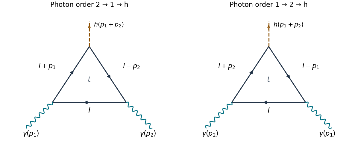
The two photon orders and consistent directed loop momenta
. Original Feynman diagrams. Solid arrows show fermion flow and the labelled internal four-momenta. Wavy external lines are incoming photons; the dashed external line is the outgoing Higgs boson. The two panels use independent dummy loop momenta. Details.In the first routing, traverse the fermion loop from the insertion to the insertion with momentum , then to the Higgs boson insertion with momentum , then back to the insertion with momentum . Conservation at the Higgs boson insertion gives . The second routing exchanges and : its three internal momenta are , and . Reversing the orientation is another way to represent this second ordering. Two vector insertions give no Furry theorem cancellation.
Past exam of the advanced fluid dynamics course of the University of Oxford 2025 2 e Solution by Codex 0 2026-10-25
Codex 0 2026-10-25For rotation about the hydrodynamic centre of a two-sphere dumbbell, the sphere centres have velocities . Their resultant drag force in the free-draining approximation isEach sphere also experiences a spin drag torque, but its isolated rotation causes no net force. Those spin contributions therefore do not alter the cancellation.
This illustrates translation-rotation reciprocal coupling. About any fixed origin, write the fluid's rigid-body force and torque asThe transposed cross-blocks follow from the Lorentz reciprocal theorem. If pure translation causes zero torque about an origin for every , then , hence pure rotation about that origin causes zero force. This implication is general for linear Stokes flow; the existence and leading location of such an origin here use the two-sphere geometry and the approximation in part c.
Past exam of the advanced fluid dynamics course of the University of Oxford 2025 2 d Solution by Codex 0 2026-10-25
Codex 0 2026-10-25Hold the two-sphere object fixed in a uniform stream . In the free-draining approximation, its drag forces are , with . The hydrodynamic torque about isTo make it zero for every incoming-stream direction, choose the hydrodynamic centre of a two-sphere dumbbell:It lies closer to the larger sphere, whose larger drag requires a shorter lever arm. Uniform translation does not spin an isolated sphere, so no additional isolated-sphere spin torque enters this leading approximation.
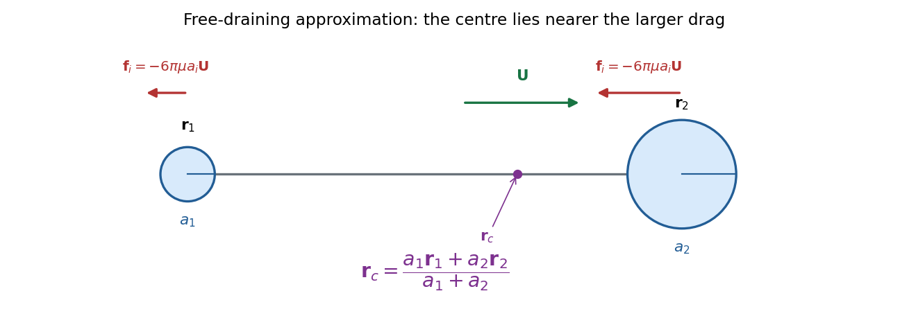
Finite-separation hydrodynamic interactions and connector drag can change the displayed location; the calculation has the same approximation as part c.
Past exam of the advanced fluid dynamics course of the University of Oxford 2025 2 c Solution by Codex 0 2026-10-25
Codex 0 2026-10-25Use the free-draining approximation: neglect the hydrodynamic interaction between the widely separated spheres and neglect the connector's viscous drag. Stokes law gives for each sphere. Their resultant isThis is the leading two-sphere approximation, not an exact finite-separation hydrodynamic resistance matrix. Writing and , the first Stokeslet reflection gives, if the connector remains negligible,The negative correction expresses reduced drag from fluid entrainment by the other sphere. A very thin but arbitrarily long rod need not have negligible total drag: its typical transverse drag scales as for rod radius . Thus the simple boxed result uses the intended negligibly dragging connector limit as well as ; the two printed size inequalities alone do not specify a uniform limit in which rod drag vanishes.
Pinned article: Introduction to the OurBigBook Project
Welcome to the OurBigBook Project! Our goal is to create the perfect publishing platform for STEM subjects, and get university-level students to write the best free STEM tutorials ever.
Everyone is welcome to create an account and play with the site: ourbigbook.com/go/register. We belive that students themselves can write amazing tutorials, but teachers are welcome too. You can write about anything you want, it doesn't have to be STEM or even educational. Silly test content is very welcome and you won't be penalized in any way. Just keep it legal!
Intro to OurBigBook
. Source. We have two killer features:
- topics: topics group articles by different users with the same title, e.g. here is the topic for the "Fundamental Theorem of Calculus" ourbigbook.com/go/topic/fundamental-theorem-of-calculusArticles of different users are sorted by upvote within each article page. This feature is a bit like:
- a Wikipedia where each user can have their own version of each article
- a Q&A website like Stack Overflow, where multiple people can give their views on a given topic, and the best ones are sorted by upvote. Except you don't need to wait for someone to ask first, and any topic goes, no matter how narrow or broad
This feature makes it possible for readers to find better explanations of any topic created by other writers. And it allows writers to create an explanation in a place that readers might actually find it.
Figure 1. Screenshot of the "Derivative" topic page. View it live at: ourbigbook.com/go/topic/derivativeVideo 2. OurBigBook Web topics demo. Source. - local editing: you can store all your personal knowledge base content locally in a plaintext markup format that can be edited locally and published either:This way you can be sure that even if OurBigBook.com were to go down one day (which we have no plans to do as it is quite cheap to host!), your content will still be perfectly readable as a static site.
- to OurBigBook.com to get awesome multi-user features like topics and likes
- as HTML files to a static website, which you can host yourself for free on many external providers like GitHub Pages, and remain in full control

Figure 2. You can publish local OurBigBook lightweight markup files to either OurBigBook.com or as a static website.
Figure 3. Visual Studio Code extension installation.
Figure 5. . You can also edit articles on the Web editor without installing anything locally. Video 3. Edit locally and publish demo. Source. This shows editing OurBigBook Markup and publishing it using the Visual Studio Code extension. 
- Infinitely deep tables of contents:




All our software is open source and hosted at: github.com/ourbigbook/ourbigbook
Further documentation can be found at: docs.ourbigbook.com
Feel free to reach our to us for any help or suggestions: docs.ourbigbook.com/#contact