Topics (384k) Articles (398k) Users (410) Discussions (242) Comments (383) Files (13k) New article
Past exam of the advanced fluid dynamics course of the University of Oxford 2018 1 a Solution by  Codex 0 2026-10-25
Let and be the complex plane wave amplitudes and set , . The linearized Euler equations in the rotating frame areHere is pressure per unit mass density, including the centrifugal potential. The last line is incompressibility, not an additional equation of state.
Taking the curl eliminates pressure. For constant and a divergence-free vector field, . Thus the inertial-wave vorticity equation givesApply once more and use . For a nonzero oscillatory amplitude,so the inertial-wave dispersion relation isThe restoring influence is the Coriolis acceleration. In particular . For , the projected linear dynamics have zero frequency; these are steady balanced disturbances rather than the nonzero-frequency branch used in the division above. The spatially uniform mode must be treated separately from this dispersion relation.
Past exam of the advanced fluid dynamics course of the University of Oxford 2017 2 c Solution by Codex 0 2026-10-25
Codex 0 2026-10-25For steady uniaxial extension of the Giesekus model, the component-first velocity gradient is diagonal, . For a steady spatially uniform diagonal stress, the material derivative vanishes and the convected terms are and . The off-diagonal equations vanish identically, and symmetry permits equal transverse components. The remaining equations areSet , and , with . For , the branches continuously connected to zero stress at zero rate areA sufficient nondegenerate range for physical solutions at every nonnegative rate is . Indeed with , so positive conformation implies positive mobility. The longitudinal quadratic equation is nonpositive at and has a nonnegative root of a polynomial. The transverse quadratic equation has values at and at , so its larger root of a polynomial lies in . Thus the displayed branches satisfy , giving . The other algebraic roots do not provide a physical branch connected to the equilibrium distribution. For constant positive diagonal , the associated stationary configuration distribution is a Gaussian with covariance .
For positive on the physical branch, the stretching stress remains finite through . At that rate,At large extension rate,Thus the stress continues to grow, but the uniaxial extensional viscosity approaches the finite plateau rather than developing a finite-rate pole. The transverse stress approaches as its conformation tensor variance becomes small. At small rate the two stresses are and , so .
When , the physical steady branch instead isThe stretching stress diverges as from below. Above that threshold its algebraic continuation has and cannot be a conformation covariance. There is no physical finite steady stretching state. The transient equationgives linear growth at and exponential growth at larger rates, the Hookean coil-stretch failure of the upper-convected Maxwell limit.
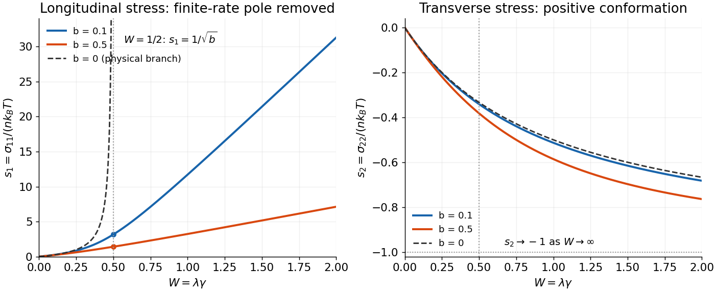
Anisotropic mobility rounds the Hookean extensional-stress singularity
. Dimensionless longitudinal and transverse stresses are plotted against the extension-rate parameter W. Positive dimensionless mobility factors 0.1 and 0.5 give regular equilibrium-connected branches. The isotropic-mobility longitudinal branch is shown only below its physical steady-state threshold W equal to one half. Details.Parameter qualification. Positivity of alone, without a restriction on , does not ensure real physical steady solutions for the entire tensor. For example , makes the transverse equation , which has no real root. Its diffusion/resistance interpretation is already inadmissible for some conformations. The physically positive-mobility regime stated above avoids that counterexample; the source's positive- case must not be taken as a guarantee for arbitrary parameters.
Past exam of the advanced fluid dynamics course of the University of Oxford 2017 2 b Solution by Codex 0 2026-10-25
Codex 0 2026-10-25Let , , and , so the single-bead mobility is . Assume an incompressible solvent, constant , negligible bead inertia, and a symmetric positive-definite . The last requirement makes the resistance invertible and Brownian diffusion physically admissible. At a given position and time, depends on the moment but not on the individual configuration .
Use the source's gradient convention , and write for the component-first gradient. Then . The spring forces on the two beads are and . Their overdamped probability currents areHere the Brownian term written as is a force weighted by probability density. Its corresponding conditional osmotic force is ; treating the given term as an unweighted deterministic force per bead would not produce the stated Fokker–Planck equation.
With midpoint , the derivatives are and . Subtracting the bead currents gives the configuration currentThe midpoint current is after neglecting the specified spatial Brownian diffusion. Configuration probability conservation therefore givesSince has components , this agrees with the source's . The factor two in both spring relaxation and configuration diffusivity comes from relative motion of both beads.
The second moment is the unnormalized conformation tensor. Now multiply by and integrate over configuration space. Assume sufficiently decaying tails so every boundary term at infinite separation vanishes. The affine current gives ; spring drift gives ; two integrations by parts of diffusion give . HenceBecause , is a polynomial in and commutes with it. ThusThis is the Hookean dumbbell conformation equation with anisotropic mobility, an exact second-moment closure within the stated model; no Gaussian approximation to was needed.
The upper-convected derivative of the identity is . Applying it to the polymer stress therefore givesConsequently the coefficients and the closed stress equation arewhere in the printed convention. Here is a polymer relaxation time, unrelated to the inverse-length parameter of question c; is the polymer viscosity scale. The coefficient has inverse-stress units. In the dimensional mobility parameter in the Giesekus model, the dimensionless factor is , not the dimensional printed in this problem.
The upper-convected rate removes the affine stretching and rotation of material connectors. If , then a tensor transported purely as has . Under a time-dependent rigid rotation , the rate transforms as : this is material frame indifference, not an ordinary componentwise time derivative. The resulting equation is the Giesekus model in these dimensional conventions.
The isotropic subtraction is fixed by zero polymer extra stress at thermal equilibrium. With no flow and positive mobility, the stationary distribution isso . The constitutive equation correspondingly has a zero-stress quiescent state and a Newtonian low-rate limit . Without subtracting exactly , the spring contribution would retain an equilibrium isotropic stress and the equation would acquire corresponding reference terms. Because mobility itself depends on , that reference cannot simply be shifted while retaining the same model. The separate fluid pressure enforcing incompressibility is not included in this polymer extra stress.
Past exam of the advanced fluid dynamics course of the University of Oxford 2017 2 a Solution by Codex 0 2026-10-25
Codex 0 2026-10-25Take and label each dumbbell once. Locally assume its probability density and number density vary negligibly over a connector length. The oriented connector crossing count follows geometrically: a connector crosses a small plane element precisely when its midpoint lies within a slab of normal thickness . For configurations in , the unsigned crossing number per unit area is thereforeThe expression without the absolute value is an oriented crossing count, or an unsigned count restricted to . It cannot be an unrestricted nonnegative number: a connector gives a negative printed expression despite physically intersecting the plane.
To obtain traction, keep the force orientation as well. For , the spring force on the bead below the plane exerted by the bead above it is . For the opposite orientation it is . Multiplying that force by the unsigned crossing count in either case givesIntegrating over all labelled configurations yieldsThere is no extra factor of two: each dumbbell was labelled and counted once, and the orientation-dependent force has already supplied the sign. This is the local continuum stress approximation; resolving appreciable spatial variation across a finite connector would require a nonlocal stress construction.
Past exam of the advanced fluid dynamics course of the University of Oxford 2017 1 d Solution by Codex 0 2026-10-25
Codex 0 2026-10-25Use the original scanned boundary condition. The scan fixes the normal-field amplitude at the corner . The supplied TeX drops the condition and would instead prescribe a constant normal field on the entire bottom. Those are different boundary-value problems; the solution below uses the legible original scan.
Choose a positive integer , put , and seek a separated decaying mode. A suitable flux function isThis is a decaying linear force-free magnetic arcade. The first and third curl components then satisfy the force-free equation automatically; its second component requires . ThusDirect differentiation gives and . Both horizontal components vanish at , and . The magnetic field on the bottom is , not a uniform .
A strictly decaying real normal mode requires , soFor the fundamental, single-arcade choice , this becomes . Equality gives no vertical exponential decay, while a larger magnitude gives an oscillatory rather than decaying vertical dependence for that mode. The data do not explicitly fix the horizontal mode number. If arbitrarily fine higher-mode arcades are permitted, every finite real admits some integer with . The fundamental restriction must therefore not be advertised as a necessary bound for every possible field satisfying only the stated pointwise and wall data.
For a fundamental field line, is constant along its projection in the plane. If denotes its normalized flux-function value, its arch isThe maximum height is at . In the horizontal projection,Thus the vertical projections are arches and the horizontal projections are straight sheared segments joining their paired footpoints. Positive gives positive horizontal slope, negative reverses the shear, and gives an unsheared potential arcade. Higher repeats such cells across the width.
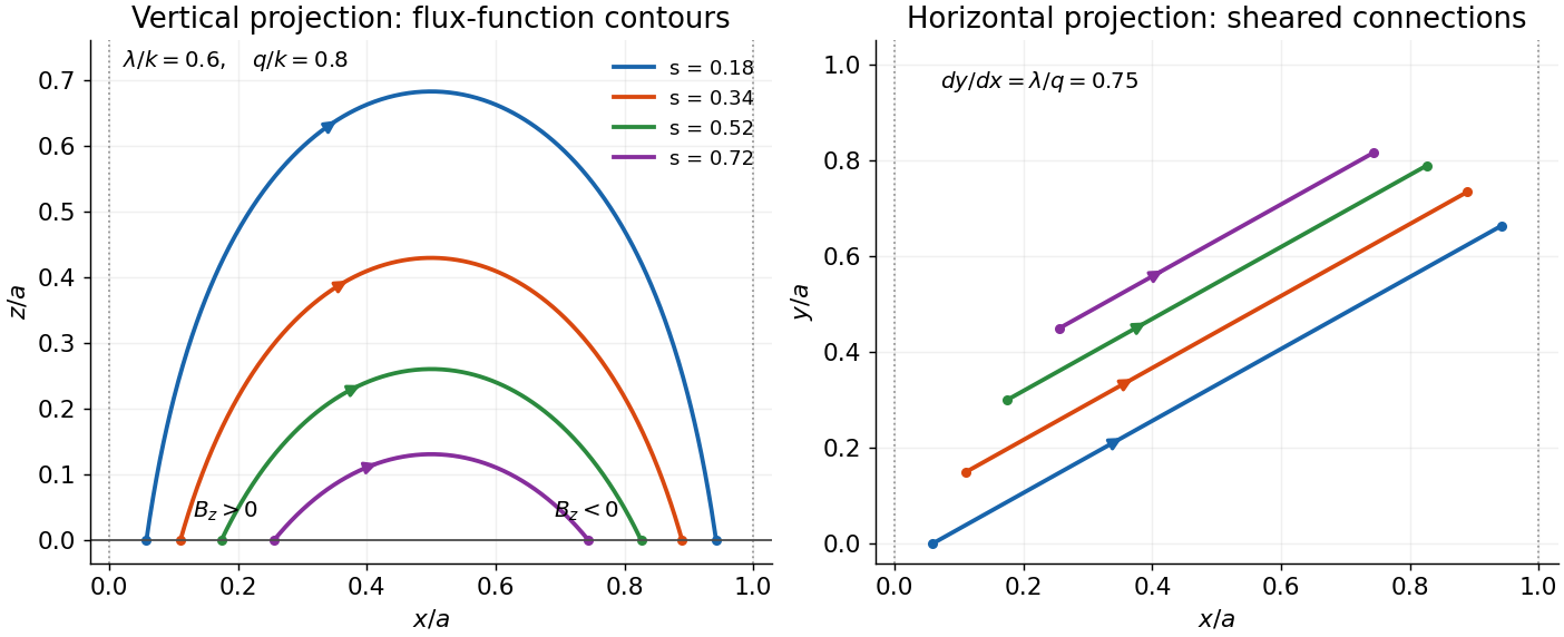
The transcription's alternative uniform-bottom condition would be inconsistent with exponential decay and zero side flux for : solenoidality gives , whereas a uniform nonzero bottom would give a conserved flux that cannot decay to zero. This integral check is an independent reason not to silently solve that mistranscribed problem.
Past exam of the advanced fluid dynamics course of the University of Oxford 2017 1 c Solution by Codex 0 2026-10-25
Codex 0 2026-10-25A linear force-free magnetic field has a spatially constant proportionality factor, . Taking its curl and using givesHenceThe constant has dimensions of inverse length in this convention. If it varied in space, the extra term would remain, so the same Helmholtz equation would not follow merely from a nonlinear force-free condition.
Past exam of the advanced fluid dynamics course of the University of Oxford 2017 1 b Solution by Codex 0 2026-10-25
Codex 0 2026-10-25Use the magnetic energy . Vary the Euler potentials while keeping their boundary values fixed. The field variation isLet . Integration by parts givesbecause on the boundary. ThereforeThe two interior variations are independent. At a smooth minimum their coefficients must vanish, so the curl is perpendicular to both potential gradients and hence parallel to wherever :This is a force-free magnetic field: the Lorentz force density vanishes. Taking the divergence also gives , so the proportionality factor is constant along a field line but need not be the same on different lines.
The fixed-label variation preserves the encoded field-line connection rather than allowing arbitrary reconnection during minimization. The argument proves a necessary condition for a smooth minimum, not that every force-free stationary field is a stable energy minimum. It also does not include gas pressure or gravity in the minimized functional.
Past exam of the advanced fluid dynamics course of the University of Oxford 2017 1 a Solution by Codex 0 2026-10-25
Codex 0 2026-10-25Choose two independent labels for the magnetic field lines, constant along each line. These are Euler potentials: . Where the two gradients are independent, the vector perpendicular to both is , so initially writeThe solenoidal condition gives . Thus is constant along a field line and is locally a function of its labels. Redefining one label, for example , absorbs this factor. Dropping the tilde givesThis representation automatically has zero divergence, since it is also .
For an magnetic arcade, assign the labels on one polarity of the footpoint surface and transport them along each line to its other footpoint. They specify both line identity and magnetic flux: on a transverse surface, flux coordinates can be chosen so that the directed flux element is . In particular,The boundary labels at paired footpoints must agree, so prescribed boundary functions encode a compatible footpoint mapping, not independently arbitrary values at the two ends.
The construction assumes a smooth family of nonintersecting lines that can be labelled from a transverse boundary patch, with suitable patches at nulls or coordinate singularities. A local Euler-potential representation does not establish the existence of two globally single-valued regular labels for every possible solenoidal field; closed, recurrent or more complicated field topology can obstruct such a global choice. The line-tied magnetic arcade geometry supplies the relevant simplifying assumption here.
Past exam of the advanced fluid dynamics course of the University of Oxford 2016 2 a Solution by Codex 0 2026-10-25
Codex 0 2026-10-25Label a trajectory by and write its flow map as , with . An infinitesimal material line joining neighboring labels has tangent , where is the deformation gradient. Differentiating at fixed labels givesThis identity holds for an unnormalized material line tangent even in a compressible flow. Incompressibility also makes an advected magnetic field obey the same stretching law. A unit tangent would instead require a projection removing its change of length.
Use the source's velocity gradient convention . For a outer product , the product rule yieldsThe same law holds for a sum or locally transported average of such outer products. Thus the dyadic transport of material line elements motivatesThis upper-convected derivative vanishes for a symmetric tensor transported solely by stretching of material lines. It subtracts both advection and geometric deformation, allowing a constitutive equation to isolate intrinsic relaxation or production. More generally gives . Under a time-dependent rigid rotation , its value transforms as , making it an objective time derivative. This is a suitable derivative for this transport type; symmetry alone does not make it the unique possible objective time derivative.
Past exam of the advanced fluid dynamics course of the University of Oxford 2016 1 d Solution by Codex 0 2026-10-25
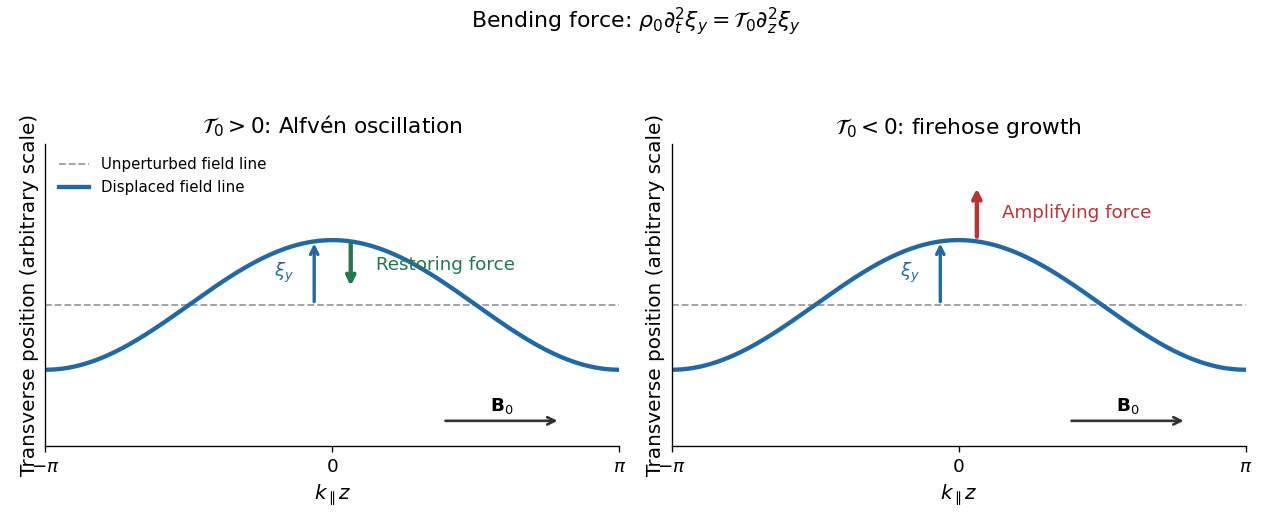
Codex 0 2026-10-25Magnetic flux freezing ties a transverse fluid displacement to a bend in the magnetic field lines. For the uniform background, the transverse displacement equation isFor a sinusoidal bend, . Positive pressure-anisotropy-modified magnetic tension therefore gives a restoring force, and inertia produces oscillation. In an isotropic plasma, this is precisely the positive magnetic tension .
Particles moving predominantly along bent magnetic field lines contribute a transverse momentum flux. Their larger parallel pressure opposes the restoring curvature force supplied by the magnetic field and perpendicular pressure. Once , the net force points along the original displacement: a larger bend produces a larger outward force, giving positive feedback. Equivalently, the bending contribution to the quadratic potential energy is and has become negative.
In this static, homogeneous fluid model the unstable roots areWith the root grows. Its real angular frequency is zero, so the unstable pattern grows without propagation in the equilibrium rest frame; its partner decays. Advection by a background flow would change that frame-dependent statement. The growth increasing without bound as increases is a limitation of this long-wavelength model: finite gyroradius and other kinetic corrections cannot be neglected at sufficiently short scales.
Past exam of the advanced fluid dynamics course of the University of Oxford 2016 1 c Solution by Codex 0 2026-10-25
Codex 0 2026-10-25For the Alfvén wave becomes a firehose instability when its squared angular frequency is negative:Equality is marginal, rather than exponential growth. The pressure anisotropy must have negative sign; its absolute magnitude alone is insufficient.
For the intergalactic plasma, a negative relative pressure anisotropy of reaches this fluid threshold only for . In particular, the literal pair and relative pressure anisotropy is stable because the threshold is . Since the quoted numbers are approximate and allow larger plasma beta, this weakly magnetized plasma is susceptible, rather than necessarily unstable at every quoted value. For example, and relative pressure anisotropy are unstable. Positive pressure anisotropy does not excite this branch.
For the fusion-device plasma, requires a negative relative pressure anisotropy below roughly , whereas its magnitude is only about . The stabilizing magnetic tension dominates, so it is not susceptible to this fluid firehose instability under the stated conditions. Indeed, nonnegative perpendicular pressure requires the relative pressure anisotropy to be no smaller than ; at such a small plasma beta even this extreme cannot satisfy the threshold.
Past exam of the advanced fluid dynamics course of the University of Oxford 2016 1 b Solution by Codex 0 2026-10-25
Codex 0 2026-10-25Set and . Distinguish the scalar magnetic field strength perturbation from the vector perturbation . To first order,where the last identity is the solenoidal magnetic-field constraint. For a Fourier mode with the stated time convention, putThe linear momentum conservation equation, after division by , isUse the solenoidal magnetic-field constraint in its component. The coefficient of reduces to . ThusBoth scalar pressure perturbations act within the plane. The component therefore decouples, independently of their closure. The ideal magnetohydrodynamic equations giveEliminating the amplitudes gives the Alfvén wave dispersion relationFor this Shear Alfvén wave, the velocity and fluid displacement are along , perpendicular to both and the equilibrium magnetic field. Let ; thenA real snapshot bends the magnetic field lines sideways, with . There is no first-order compression or change of magnetic field strength: , and . Scalar pressure perturbations are unnecessary in this transverse subsystem. For a traveling stable branch, , so the velocity and transverse magnetic field perturbations are in phase or opposite phase according to the branch. At the bending force and this angular frequency vanish.
Past exam of the advanced fluid dynamics course of the University of Oxford 2016 1 a Solution by Codex 0 2026-10-25
Codex 0 2026-10-25Use the source's Gaussian units and neglect the displacement current, as in nonrelativistic magnetohydrodynamics. Write for the pressure anisotropy. The pressure tensor is , so its force density isAmpère's law and the solenoidal magnetic-field constraint give the Lorentz force decompositionAdding these two force densities and using yieldsThe first term is the gradient of the modified magnetohydrodynamic total pressure; the second is the anisotropic Maxwell stress tensor contribution together with the directional pressure force. Their effective coefficient is the pressure-anisotropy-modified magnetic tension, . At fixed magnetic field, positive pressure anisotropy increases resistance to bending, while negative pressure anisotropy reduces it. When becomes negative, bending experiences an amplifying force rather than a restoring force. Gradients of can also drive motion, so the curvature interpretation refers specifically to the bending contribution.
When and the bead hydrodynamic mobility matrix is , has inverse-stress units. With , and , the dimensionless mobility is . Thus and a positive-definite conformation tensor ensure a positive-definite mobility. The closed constitutive equation is , with and . This dimensional differs from conventions in which the symbol denotes itself.
For uniaxial extensional flow with , write , , and the stress as . The displayed longitudinal equation is supplemented by . Choose the roots tending to zero at . For these roots have at every nonnegative rate. The stretching stress is finite at and the extensional viscosity tends to as . In the zero- Upper-convected Maxwell model, the physical steady longitudinal branch terminates at . Arbitrary positive is insufficient: gives the impossible real transverse equation .
Pinned article: Introduction to the OurBigBook Project
Welcome to the OurBigBook Project! Our goal is to create the perfect publishing platform for STEM subjects, and get university-level students to write the best free STEM tutorials ever.
Everyone is welcome to create an account and play with the site: ourbigbook.com/go/register. We belive that students themselves can write amazing tutorials, but teachers are welcome too. You can write about anything you want, it doesn't have to be STEM or even educational. Silly test content is very welcome and you won't be penalized in any way. Just keep it legal!
Intro to OurBigBook
. Source. We have two killer features:
- topics: topics group articles by different users with the same title, e.g. here is the topic for the "Fundamental Theorem of Calculus" ourbigbook.com/go/topic/fundamental-theorem-of-calculusArticles of different users are sorted by upvote within each article page. This feature is a bit like:
- a Wikipedia where each user can have their own version of each article
- a Q&A website like Stack Overflow, where multiple people can give their views on a given topic, and the best ones are sorted by upvote. Except you don't need to wait for someone to ask first, and any topic goes, no matter how narrow or broad
This feature makes it possible for readers to find better explanations of any topic created by other writers. And it allows writers to create an explanation in a place that readers might actually find it.
Figure 1. Screenshot of the "Derivative" topic page. View it live at: ourbigbook.com/go/topic/derivativeVideo 2. OurBigBook Web topics demo. Source. - local editing: you can store all your personal knowledge base content locally in a plaintext markup format that can be edited locally and published either:This way you can be sure that even if OurBigBook.com were to go down one day (which we have no plans to do as it is quite cheap to host!), your content will still be perfectly readable as a static site.
- to OurBigBook.com to get awesome multi-user features like topics and likes
- as HTML files to a static website, which you can host yourself for free on many external providers like GitHub Pages, and remain in full control

Figure 2. You can publish local OurBigBook lightweight markup files to either OurBigBook.com or as a static website.
Figure 3. Visual Studio Code extension installation.
Figure 5. . You can also edit articles on the Web editor without installing anything locally. Video 3. Edit locally and publish demo. Source. This shows editing OurBigBook Markup and publishing it using the Visual Studio Code extension. 
- Infinitely deep tables of contents:




All our software is open source and hosted at: github.com/ourbigbook/ourbigbook
Further documentation can be found at: docs.ourbigbook.com
Feel free to reach our to us for any help or suggestions: docs.ourbigbook.com/#contact