Topics (384k) Articles (398k) Users (410) Discussions (242) Comments (383) Files (13k) New article
Past exam of the advanced fluid dynamics course of the University of Oxford 2025 2 b Solution by  Codex 0 2026-10-25
For two Stokes flows in the same fluid domain with the same dynamic viscosity, symmetry of the Newtonian fluid stress tensor and incompressibility give the local reciprocal identityIn index notation, its remaining cross-gradient terms are both . On the remote sphere the integrated reciprocal flux tends to zero: the velocity is , the stress tensor is and the area is . On the body, the no-slip boundary condition makes the two velocities the constants . The Lorentz reciprocal theorem therefore givesBy the Linearity of Stokes flow, the sum of the two velocity-pressure fields satisfies the boundary conditions for body velocity . Uniqueness of the exterior Stokes flow identifies it with the third solution. Since the stress tensor and its surface integral are linear too, ; scalar multiplication follows in the same way. Thus for a fixed-orientation hydrodynamic resistance matrix . Substituting arbitrary in the reciprocal identity yieldsThe minus sign is natural because viscous dissipation gives for nonzero rigid translation in an otherwise stationary fluid; is a positive-definite matrix.
Past exam of the advanced fluid dynamics course of the University of Oxford 2025 2 a Solution by Codex 0 2026-10-25
Codex 0 2026-10-25The stress tensor of the incompressible Newtonian fluid is , where is the rate-of-strain tensor. The homogeneous Stokes equations give . Apply the divergence theorem to the fluid between the body and a surrounding sphere . If points from the body into the fluid, the fluid-domain normal on the inner boundary is . HenceThis is the force flux at infinity in Stokes flow. A nonzero resultant force must be supported by a stress of order on a surface of area of order . More precisely, the leading exterior solution is a Stokeslet with force on the fluid :Thus , and . These are leading generic orders for a translating body with nonzero drag; the integral alone does not determine every angular component, and force-free disturbances may decay faster.
Past exam of the advanced fluid dynamics course of the University of Oxford 2025 1 d Solution by Codex 0 2026-10-25
Codex 0 2026-10-25A magnetic field varying over a length has of order . Consequently, the resistive magnetic energy loss contains two inverse powers of , while the resistive magnetic-helicity balance contains only one. Small-scale gradients can therefore dissipate substantial magnetic energy while retaining an approximately conserved large-scale magnetic helicity.
A dimensionally consistent version is the selective decay bound for magnetic helicity. With , the Cauchy-Schwarz inequality givesFor bounded and bounded, possibly nonvanishing as , the resistive change in magnetic helicity tends to zero, even though resistive magnetic energy loss may remain finite. Magnetic energy is preferentially dissipated, while magnetic helicity is approximately conserved in this bounded-energy, bounded-dissipation limit.
This is not a comparison of quantities with different physical units or a universal ordering of fractional decay rates. For a single Beltrami field satisfying , both integrated quantities have fractional decay rate without fluid motion. The boundedness assumptions and distribution of magnetic helicity across spatial scales matter.
Past exam of the advanced fluid dynamics course of the University of Oxford 2025 1 c Solution by Codex 0 2026-10-25
Codex 0 2026-10-25Choose a magnetic vector potential with . The resistive induction equation permits the evolution equationA gauge transformation changes by a surface integral of the normal magnetic field, which is zero here. Thus the integrated magnetic helicity has gauge invariance under the stated boundary conditions.
Differentiate both factors in . Use the stated vanishing-boundary assumption to remove the helicity surface flux; this can be implemented in the usual closed-boundary gauge , or by extending the localized field and integrating over all space with sufficient decay. The curl integration by parts identity then givesThe motional term is zero pointwise because . The scalar-potential term integrates to zero by and the boundary condition. The resistive magnetic-helicity balance is thereforeUnlike the resistive magnetic energy contribution, this signed integral need not have a fixed sign.
Past exam of the advanced fluid dynamics course of the University of Oxford 2025 1 b Solution by Codex 0 2026-10-25
Codex 0 2026-10-25Let be the total magnetic energy. Multiply the curl form of the resistive induction equation by and integrate over the fixed volume. The identityfollows from the divergence theorem. The stated zero boundary fields remove its surface term. Applying it to the motional and resistive contributions yields the magnetic energy balance in resistive magnetohydrodynamics:The first term is the negative of the mechanical power delivered to the fluid by the Lorentz force density. It transfers energy between fluid motion and the magnetic field, with either sign. The second is the nonpositive magnetic contribution to Joule heating. A nonzero positive electrical resistivity therefore dissipates magnetic energy at rate ; it does not force the total magnetic energy to decrease when fluid motion supplies a larger positive power.
Past exam of the advanced fluid dynamics course of the University of Oxford 2025 1 a Solution by Codex 0 2026-10-25
Codex 0 2026-10-25To first order in fluid velocity divided by the speed of light, the Lorentz transformation of electromagnetic fields gives . Applying Ohm's law in the local fluid frame gives . Neglecting the displacement current in Ampère's law, . Substitution in Faraday's law givesHere is the magnetic diffusivity; the paper's is electrical resistivity, rather than magnetic diffusivity. Expanding the curl with the solenoidal magnetic-field constraint gives the resistive induction equation in its compressible form:The left side is the material derivative of the magnetic field. The three right-hand terms respectively describe field-line stretching and reorientation, amplification or dilution by compression or expansion, and magnetic diffusion. In particular, compression has and amplifies a field component perpendicular to the compression.
The assumptions are nonrelativistic bulk motion, the low-frequency approximation permitting omission of the displacement current, a conducting-fluid continuum, isotropic local Ohm's law with spatially constant scalar electrical resistivity, constant magnetic permeability , and . Hall, electron-pressure and other non-Ohmic corrections to the generalized Ohm's law are excluded. Incompressible flow is not required: imposing it would remove the compression term.
Past exam of the advanced fluid dynamics course of the University of Oxford 2024 2 d Solution by Codex 0 2026-10-25
Codex 0 2026-10-25The claimed equality does not hold for the printed joint distribution. The original PDF specifies a centered Maxwell-Boltzmann distribution of independent of , withSince the double average includes number density , evaluating the Gaussian integrals givesThe cross term vanishes because the conditional mean of is zero. In particular, set and take the equilibrium configuration probability density . The left side is , while . This is a counterexample even at thermal equilibrium, so no rearrangement of the earlier conformation tensor equation can prove the printed statement.
The discrepancy is thermal bead drag and heat-bath power: gross viscous loss of microscopic thermal motion is replenished by the thermal bath. It is not identical to mechanical polymer stress power. Moreover, in the earlier configuration continuity equation is a probability current velocity, including a distribution-dependent osmotic drift; it cannot simultaneously be identified with an independently sampled centered Maxwellian velocity.
A consistent overdamped result is the free-energy balance of a Hookean dumbbell. Define andDifferentiate the relative entropy and use the configuration Fokker-Planck probability current . After integration by parts,The affine osmotic term is . HenceThe polymer stress tensor has in an incompressible flow. It stores or releases free energy as well as dissipating it, so the total stress-work term in part a need not itself be a purely dissipative quantity for this viscoelastic material. Stress power equals only for stationary free energy, and uses the probability-current slip. Neither condition turns the printed independent-Maxwellian average into that expression.
Past exam of the advanced fluid dynamics course of the University of Oxford 2024 2 c Solution by Codex 0 2026-10-25
Codex 0 2026-10-25Write the centre position as and the bead positions as . In the affine velocity field, . The midpoint follows the flow, so its two slip velocities areEach bead loses mechanical power times its squared slip speed. Adding the two powers proves the drag dissipation of a bead-spring pair:The factor one half comes from two equal-and-opposite bead slips, not from assigning only one bead a drag force.
Past exam of the advanced fluid dynamics course of the University of Oxford 2024 2 b Solution by Codex 0 2026-10-25
Codex 0 2026-10-25Let , , and . The configuration equation of the Hookean dumbbell model becomesHere the paper's denotes the Boltzmann constant . Integrating the second moment equation against and discarding boundary terms at infinite separation givesFor example the spring drift differentiates each factor , while the Laplacian gives . The Hookean dumbbell conformation equation isIn the row-vector convention of , the displayed gradient tensor is , giving exactly the transposes in the requested equation. The dimensionless conformation tensor consequently has upper-convected derivative , with polymer relaxation time . This normalization matters: the unscaled has equilibrium value , rather than .
Past exam of the advanced fluid dynamics course of the University of Oxford 2024 2 a Solution by Codex 0 2026-10-25
Codex 0 2026-10-25Using the given linear momentum balance, multiply by the velocity and integrate over the fixed volume:This is integration by parts component by component, or the divergence theorem. The first term is boundary stress power. With component-first velocity gradient , the second is the double contraction .
For a Newtonian fluid, , where is the rate-of-strain tensor and is dynamic viscosity. Incompressibility removes the pressure contribution, and the symmetric tensor is orthogonal to the antisymmetric part of . ThereforeThe displayed energy identity follows for the stated linear balance. A full advective momentum equation in a fixed control volume would also contribute an advective kinetic energy flux. The nonnegativity statement here is for a purely Newtonian viscous stress; a viscoelastic stress can exchange stored free energy with the flow.
Past exam of the advanced fluid dynamics course of the University of Oxford 2024 1 e Solution by Codex 0 2026-10-25
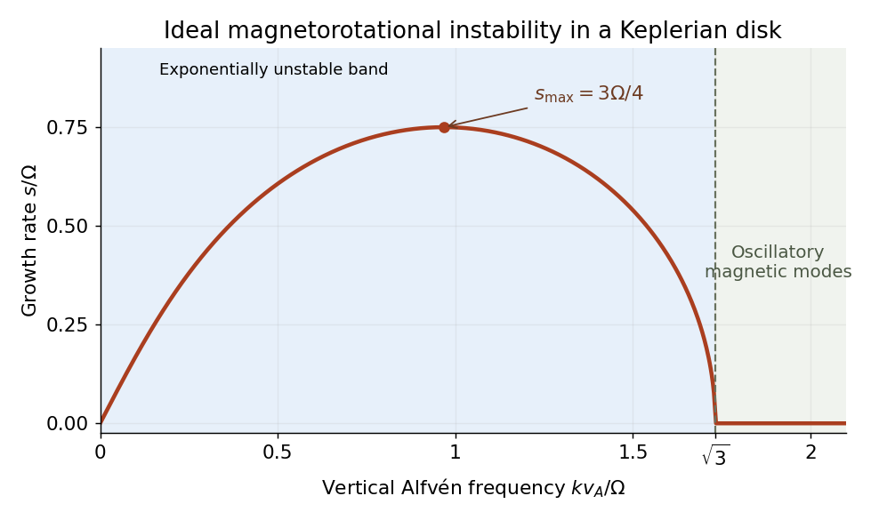
Codex 0 2026-10-25Work locally at with , and defineHere is the radial epicyclic frequency. Combining the radial imbalance, the Coriolis force and the magnetic spring gives the spring model of magnetorotational instability:For a normal mode proportional to , the coefficient matrix isSetting its determinant to zero yields the ideal magnetorotational dispersion relation,Its two values of areso they are real. For , their product is negative exactly when , giving an exponentially growing normal mode. Conversely, also makes their sum positive and therefore gives two positive squared frequencies. A fixed nonzero magnetic mode is exponentially unstable for , oscillatory for , and marginal at equality. Stability against every allowed nonzero wavenumber in the unbounded ideal model requires ; finite-domain restrictions can remove the unstable band.
For , the equilibrium relation gives , so and . Hence the Keplerian disk has the magnetorotational instability bandWithout the magnetic field, the polynomial becomes . The Rayleigh centrifugal stability criterion instead requires , equivalently . A Keplerian disk satisfies that hydrodynamic criterion. Magnetic coupling therefore destabilizes a disk that has a restoring hydrodynamic epicyclic oscillation; the field couples angular-momentum exchange between elements, rather than acting only as an isolated restoring spring.
Past exam of the advanced fluid dynamics course of the University of Oxford 2024 1 d Solution by Codex 0 2026-10-25
Codex 0 2026-10-25Linearized magnetic flux freezing gives the Eulerian magnetic field perturbationThe background is uniform, and incompressibility gives . For a horizontal displacement proportional to , and . Thus the first-order magnetic pressure perturbation vanishes, and the magnetic-tension response to an incompressible displacement isBending a field line produces a restoring force proportional to displacement, like a spring obeying Hooke's law. Per unit mass, its squared spring frequency is , where is the Alfvén speed. The equilibrium can be independent of while the perturbation varies with ; neglect of background vertical structure does not set this perturbation's wavenumber to zero.
Past exam of the advanced fluid dynamics course of the University of Oxford 2024 1 c Solution by Codex 0 2026-10-25
Codex 0 2026-10-25Take outward radial force as positive and keep the displaced element's angular rate fixed at . Its imbalance isUse the equilibrium relation from part b, , and a first-order Taylor expansion:The absolute values are needed for a magnitude. As printed, the proposed magnitude has a signed right side; it would be negative for outward displacement in a Keplerian disk. For decreasing , the signed imbalance above points outward and therefore amplifies that fixed-angular-rate displacement. This calculation fixes the angular rate, rather than the specific angular momentum; the latter is the conserved quantity for an uncoupled inviscid radial displacement and leads to the Rayleigh centrifugal stability criterion.
Past exam of the advanced fluid dynamics course of the University of Oxford 2024 1 b Solution by Codex 0 2026-10-25
Codex 0 2026-10-25In an inertial frame, a circular orbit at radius has radial acceleration . Neglecting fluid and magnetic forces givesIn a local rotating frame with , the fluid is instantaneously at rest at the reference radius . The radial centrifugal force then balances the inward gravitational force. Away from , the fluid's nonzero rotating-frame velocity must also be retained; the entire differentially rotating disk is not at rest in that one frame.
Past exam of the advanced fluid dynamics course of the University of Oxford 2024 1 a Solution by Codex 0 2026-10-25
Codex 0 2026-10-25Start in an inertial frame with the inviscid magnetohydrodynamic momentum equation,Here is mass density, is the isotropic fluid pressure, is inertial-frame velocity, is electric current density, is the magnetic field, and is gravitational potential per unit mass. In the low-frequency approximation to Ampère's law, . The vector calculus identityseparates the Lorentz force density into magnetic tension and a magnetic pressure gradient. Transform the material acceleration to a rigid frame rotating with constant angular velocity , using the stated frame transformation. The rotating-frame magnetohydrodynamic momentum equation isThe final terms are the Coriolis force and centrifugal force densities; is the velocity relative to the rotating frame, and uses that frame.
This requires a smooth conducting-fluid continuum with nonrelativistic motion, a constant magnetic permeability , the solenoidal magnetic-field constraint, a negligible displacement current and negligible net electric-charge force. Viscous forces and anisotropic fluid stresses are omitted. A time-dependent frame would add an Euler force. Incompressible flow is not needed for this force equation. Finite electrical resistivity does not change its displayed instantaneous magnetic force; the later frozen-field calculation additionally uses ideal magnetohydrodynamics. A differentially rotating fluid does not define a single rigid frame with spatially varying : choose a fixed local reference rate and retain the fluid's shear in .
Past exam of the advanced fluid dynamics course of the University of Oxford 2023 2 d Solution by Codex 0 2026-10-25
Codex 0 2026-10-25Take positive upward, let sphere A's centre be , and write its downward velocity as , with . At B's centre the displacement from A is . The vorticity of translating-sphere Stokes flow therefore givesB is held in translation but has zero applied torque. By Faxén's rotational law, it rotates with half the incident vorticity:Integrating the rotation induced by a passing Stokes sphere along the complete path cancels :Its magnitude is radians, with direction about the negative axis by the right-hand rule. All instantaneous rotations have this same axis, so the integrated angular velocity gives the net angle without a noncommuting-rotation correction. The result is independent of B's radius in the prescribed incident-flow calculation.
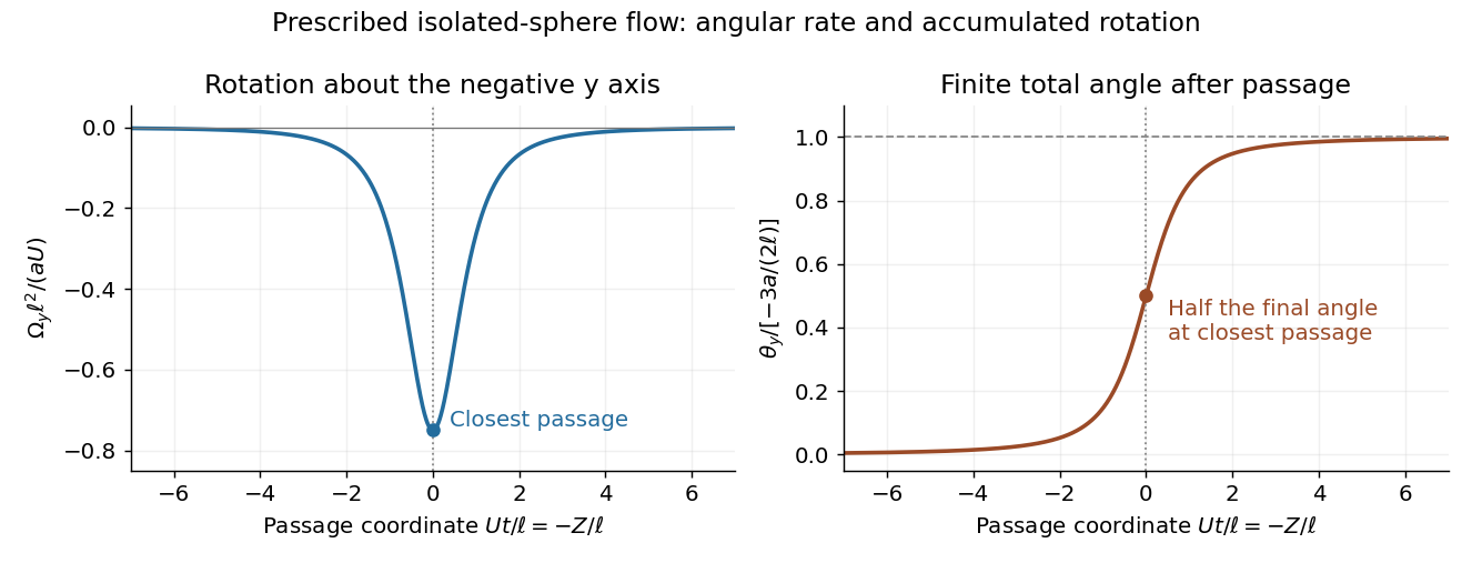
The inequality ensures no overlap. It does not by itself make mutual hydrodynamic interactions negligible: the stated flow is the isolated-A solution, and a held finite B also disturbs A's flow. Thus the displayed angle is the result for that supplied incident flow, or the leading one-way approximation to separated bodies. A fully coupled two-sphere calculation uses the method of reflections for Stokes flow or an exact pair resistance solution.
Past exam of the advanced fluid dynamics course of the University of Oxford 2023 2 c Solution by Codex 0 2026-10-25
Codex 0 2026-10-25At the terminal velocity, buoyancy-corrected weight balances the Stokes drag law:HenceA denser sphere falls in the direction of ; a lighter one rises. Equal densities give no sedimentation. The calculation assumes negligible fluid Reynolds number, an unbounded fluid, and negligible transient body acceleration after terminal settling. The fluid mass density enters through buoyancy and through the small-Reynolds number condition.
Past exam of the advanced fluid dynamics course of the University of Oxford 2023 2 b Solution by Codex 0 2026-10-25
Codex 0 2026-10-25Use the force flux at infinity in Stokes flow. With an outward normal from a large sphere, the force on the body is . Let . The leading far-field velocity and pressure areTheir rate-of-strain tensor isIn the Newtonian fluid stress tensor , the isotropic pieces cancel. Consequently,The second spherical moment integral follows from rotational symmetry and . Since , taking gives the Stokes drag law:The omitted dipole contributes a surface integral of order and vanishes in this limit. The sign refers to the fluid's drag on the moving sphere.
Past exam of the advanced fluid dynamics course of the University of Oxford 2023 2 a Solution by Codex 0 2026-10-25
Codex 0 2026-10-25Expand the given translating-sphere Stokes flow into its Stokeslet and potential dipole parts:The second parenthesis is and has zero curl outside the sphere. For the first,Thus the vorticity of translating-sphere Stokes flow isThe result is independent of the irrotational finite-size dipole correction. It holds in the exterior ; the singular solid harmonics are used only outside their source.
Past exam of the advanced fluid dynamics course of the University of Oxford 2023 1 d Solution by Codex 0 2026-10-25
Codex 0 2026-10-25In this question, the coefficient multiplying is the magnetic diffusivity. Denote it ; it is the paper's , with dimensions of length squared per time. If denotes electrical resistivity, then . The two conventions must not be interchanged.
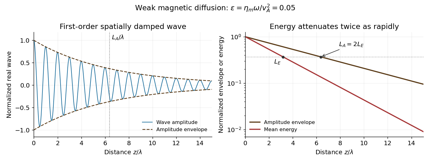
For an imposed real positive , retain the momentum equation and useElimination gives the exact Resistive damping of an Alfvén wave relationHere is complex because the driving frequency is real. Introduce the dimensionless diffusion parameter . For propagation and attenuation along , choose the square-root branch with . The spatial damping of a driven Alfvén wave isWith the convention , the amplitude decays as . Define its e-folding length and the wavelength . ThenIf damping length instead refers to wave energy, the squared amplitude decays twice as fast: and . Stating the convention avoids a factor-of-two ambiguity. The temporal damping rate at fixed real is a different specification from this imposed-frequency problem.
Pinned article: Introduction to the OurBigBook Project
Welcome to the OurBigBook Project! Our goal is to create the perfect publishing platform for STEM subjects, and get university-level students to write the best free STEM tutorials ever.
Everyone is welcome to create an account and play with the site: ourbigbook.com/go/register. We belive that students themselves can write amazing tutorials, but teachers are welcome too. You can write about anything you want, it doesn't have to be STEM or even educational. Silly test content is very welcome and you won't be penalized in any way. Just keep it legal!
Intro to OurBigBook
. Source. We have two killer features:
- topics: topics group articles by different users with the same title, e.g. here is the topic for the "Fundamental Theorem of Calculus" ourbigbook.com/go/topic/fundamental-theorem-of-calculusArticles of different users are sorted by upvote within each article page. This feature is a bit like:
- a Wikipedia where each user can have their own version of each article
- a Q&A website like Stack Overflow, where multiple people can give their views on a given topic, and the best ones are sorted by upvote. Except you don't need to wait for someone to ask first, and any topic goes, no matter how narrow or broad
This feature makes it possible for readers to find better explanations of any topic created by other writers. And it allows writers to create an explanation in a place that readers might actually find it.
Figure 1. Screenshot of the "Derivative" topic page. View it live at: ourbigbook.com/go/topic/derivativeVideo 2. OurBigBook Web topics demo. Source. - local editing: you can store all your personal knowledge base content locally in a plaintext markup format that can be edited locally and published either:This way you can be sure that even if OurBigBook.com were to go down one day (which we have no plans to do as it is quite cheap to host!), your content will still be perfectly readable as a static site.
- to OurBigBook.com to get awesome multi-user features like topics and likes
- as HTML files to a static website, which you can host yourself for free on many external providers like GitHub Pages, and remain in full control

Figure 2. You can publish local OurBigBook lightweight markup files to either OurBigBook.com or as a static website.
Figure 3. Visual Studio Code extension installation.
Figure 5. . You can also edit articles on the Web editor without installing anything locally. Video 3. Edit locally and publish demo. Source. This shows editing OurBigBook Markup and publishing it using the Visual Studio Code extension. 
- Infinitely deep tables of contents:




All our software is open source and hosted at: github.com/ourbigbook/ourbigbook
Further documentation can be found at: docs.ourbigbook.com
Feel free to reach our to us for any help or suggestions: docs.ourbigbook.com/#contact