Topics (384k) Articles (398k) Users (410) Discussions (242) Comments (383) Files (13k) New article
Past exam of the relativity course of the University of Cambridge 2015 Paper 1 4 Solution by  Codex 0 2026-10-20
Put , where , and work in the orbital plane. A dot denotes an affine-parameter derivative; for a material particle choose that parameter to be proper time.
First integrals and normalization. The geodesic Lagrangian isTime translation and axial rotation make and cyclic, givingThe tangent norm is constant along an affine geodesic because the Levi-Civita connection preserves the metric. ThereforeFor proper-time parametrization of a timelike worldline this norm is . For a null geodesic it is zero, for every affine normalization. Thus for the chosen material-particle normalization and for light. Proper time cannot itself parametrize a null ray, despite the same printed symbol being used for its affine parameter.
Null normalization and impact parameter. Under with , both and scale as , while the null path is unchanged. Their ratio is invariant. At large radius the spatial speed with respect to asymptotic time is , and orbital angular momentum per affine tangent givesFor an orientation chosen with , this is . Setting is a choice of affine scale, not a claim that all photons have equal measured energy. Once a tangent is identified with a physically normalized four-momentum, its energy fixes that scale.
Orbit shape. Substituting the constants in the norm and multiplying by givesFor and , . HenceThe radial orbit must be treated with the radial equation, because azimuth is then constant.
Circular photons and stability. For a null ray define . Its radial equation becomesThe circular orbit requires and , soIt is at a maximum of the null effective potential and is unstable. Equivalently the Binet equation linearizes about to , admitting exponentially growing radial deviations in azimuth.
Capture from infinity. Divide the null radial equation by . The quantity opposing inward motion is , whose exterior maximum is . There is no outer radial turning point precisely whenAt equality an exactly critical ray from infinity asymptotes to the photon sphere; it does not cross the horizon at a finite affine parameter. Above the threshold an initially inward ray from infinity reaches an outer turning point and scatters. The radial case is also captured. These statements refer to inward rays launched from the asymptotically flat exterior, not arbitrary initial data inside the angular-momentum barrier.
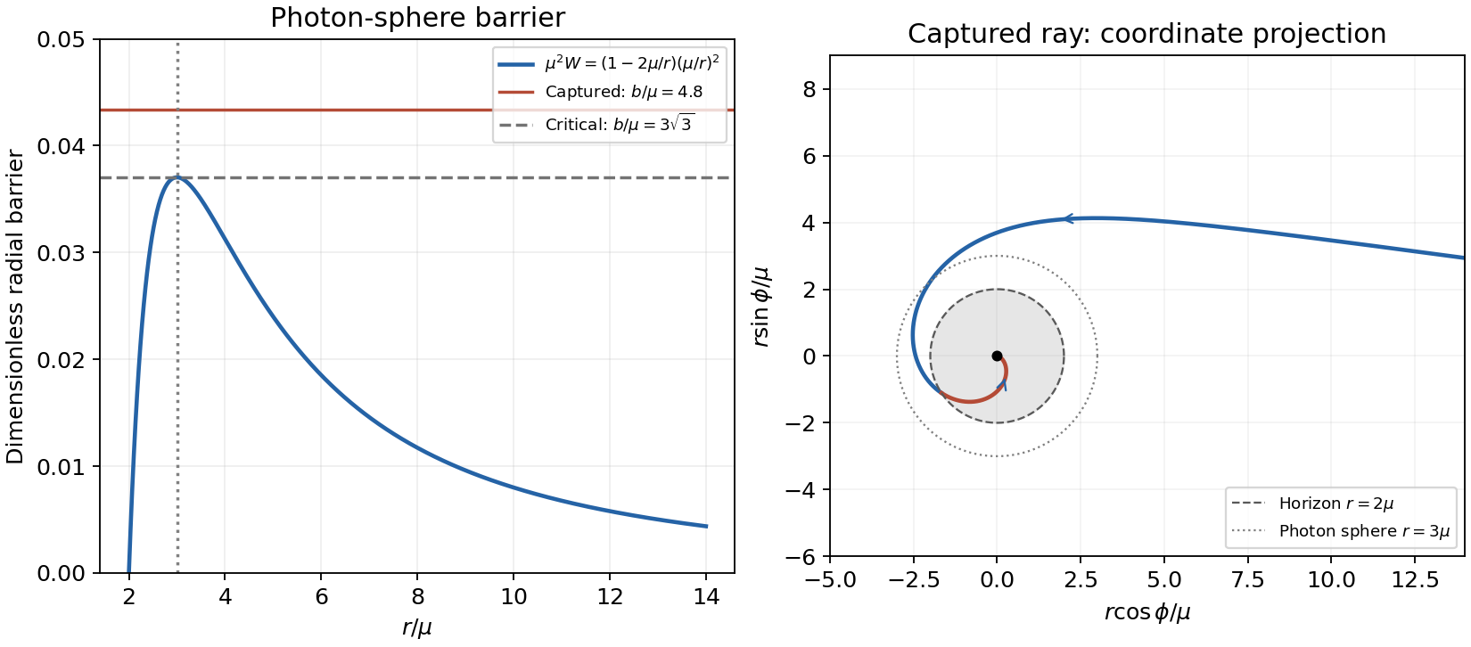
Original Schwarzschild capture calculation: the null-potential barrier and a captured equatorial ray crossing the horizon and ending at finite azimuth
. Details. Approach to the singularity. A captured nonradial ray bends inward, crosses and then the event horizon , and continues toward the curvature singularity. A plot in is only a coordinate projection, not a Euclidean spatial slice inside the horizon. For large the cubic term in the shape equation dominates:for the inward branch with . Its integral isThus the azimuth tends to a finite limit at the singularity, rather than winding infinitely often there. Near-critical rays can accumulate many turns near before capture, which is a separate phenomenon. A strictly radial ray has constant azimuth and does not admit this azimuthal asymptotic form. The radial equation also gives for a nonradial null ray, confirming finite remaining affine parameter.
Material capture and the condition at infinity. To recover the quoted threshold, take the usual marginally bound orbit, initially at rest at infinity: . With ,The turning-point quadratic has discriminant . It is positive for large and has no real positive root when , while the radial case also falls in. ThereforeAt equality the quadratic is proportional to and the orbit asymptotes to the unstable marginally bound circular orbit at . For larger , an incoming marginally bound particle encounters the outer turning point and scatters.
The source says only “from infinity”, without explicitly fixing the asymptotic speed. For a general incoming speed , andThe same bound remains sufficient for capture, since the added constant is nonnegative. It is the exact threshold only for . At fixed , the critical unstable orbit satisfiesThen . This states both the printed sufficient condition and the additional assumption needed to call it a sharp capture boundary.
Past exam of the relativity course of the University of Cambridge 2015 Paper 1 3 Solution by Codex 0 2026-10-20
Codex 0 2026-10-20Use Cartesian coordinates with and . Spatial dot and cross products below use the Euclidean three-metric. The alternating tensor is given the orientation .
Vector and covector transformation. The vector is independent of coordinates, and the chain rule gives . Likewise the one-form is independent of coordinates. Comparing coefficients provesTheir contraction is unchanged because the forward and inverse Jacobians cancel. Here lowering an index uses the metric, not an identification of the numerical upper and lower components.
Why antisymmetrization matters. Write . Differentiating the covector law givesThe last term obstructs the general tensor transformation law. It is symmetric in , so it cancels from . ThereforeEquivalently is the exterior derivative of the electromagnetic four-potential one-form. The statement that is not a tensor needs a qualification: under affine Cartesian Lorentz transformations it does transform tensorially, because the second derivatives vanish. The failure concerns arbitrary nonlinear coordinate changes, including curvilinear coordinates in flat spacetime. This distinction is precisely the difference between general covariance and covariance under the restricted inertial-frame transformations.[ref]
Lecture Notes on General Relativity by Sean M. Carroll. Section 2, Manifolds, equations 2.26–2.27: the extra second-derivative term and its cancellation under antisymmetrization
Electric and magnetic components. Choose , so , and . ThenThus the lower-index field tensor isThis is a derived component representation of the field, with the source's sign convention.
Raised indices and the first invariant. Raising both indices changes the time-space signs and leaves the spatial block unchanged:In the scalar contraction, each independent antisymmetric pair is counted twice, givingUnder a Lorentz transformation each inverse transformation from a lower index cancels its matching transformation from an upper index, leaving the same scalar. In particular a plane electromagnetic wave has in these units and makes this invariant vanish, while a pure electric field makes it negative.
The printed dual convention. The PDF explicitly defines , with no . Each independent pair therefore contributes twice: for example . The complete result isThe time-space pairs contribute and the spatial pairs contribute another . The conventional Hodge dual includes and would instead give the contraction ; it must not silently replace this paper's definition. With fixed orientation the latter contraction is a pseudoscalar: invariant under proper Lorentz transformations but odd under orientation reversal if compared using a fixed alternating symbol.
Energy density and flux. Substitution into the given mixed stress-energy tensor yieldsFor the first formula, and . For the second, . The minus sign on arises from its lowered spatial index; it does not reverse the physical energy flow. Raising that index gives , and symmetry gives , with the Poynting vector in units. Thus is energy density and represents energy flux. In SI coordinates , restore and , with . This keeps the mixed-index signs and the units distinct.
Past exam of the relativity course of the University of Cambridge 2014 Paper 1 4 Solution by Codex 0 2026-10-20
Codex 0 2026-10-20geodesic integrals and affine normalization. Put . Choose the affine parameter to be proper time, so . Cyclic and in the geodesic Lagrangian give and . Substituting into the four-velocity normalization giveshenceAn arbitrary constant rescaling of affine parameter changes its normalization; the displayed unit constant assumes the proper-time choice.
circular orbit. Define . The radial geodesic equation is . A circular geodesic therefore needs , not merely at an instant. Solving and substituting into the radial first integral givesExistence requires . circular orbits below are radially unstable, although they still define the instantaneous comparison here.
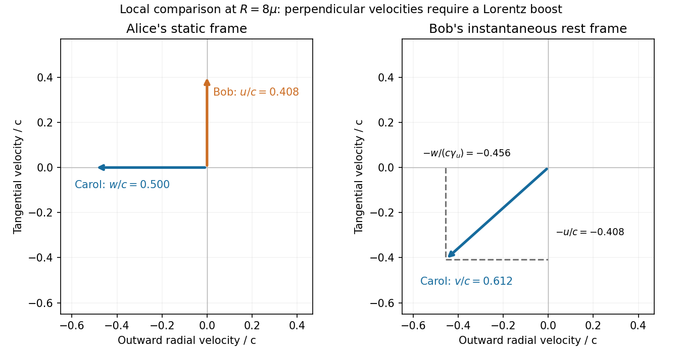
orthogonal local velocities in Schwarzschild spacetime. Use Alice's static orthonormal frame at the meeting event. Her proper clock is and tangential proper distance is . Bob's local tangential speed isCarol has and , because she starts from rest at infinity. The radial integral gives . Her static-frame radial speed is , and , soThis is inward radial motion, perpendicular to Bob's tangential motion in Alice's frame.
Special-relativistic consistency. Let Bob's tangential velocity in Alice's local frame be and Carol's inward radial speed be . A boost to Bob's frame gives Carol components and . ConsequentlyThus the three measured relative speeds agree with local Lorentz velocity addition. Ordinary Euclidean subtraction of the two velocity vectors would omit the transverse-velocity transformation.
Past exam of the relativity course of the University of Cambridge 2014 Paper 1 3 Solution by Codex 0 2026-10-20
Codex 0 2026-10-20Boost and velocity transformation. For the moving frame,The inverse has . Taking differentials of that inverse and dividing by gives
Constant proper acceleration. For collinear motion, the instantaneous rest-frame acceleration is . Since ,Write ; then . Starting from rest gives , and . integration with the stated initial origin yields
photon rocket mass ratio. In the instantaneous rest frame, ejecting backward photon energy gives, to first order, and . Hence , andHere includes all stored fuel and energy. This assumes complete conversion into a perfectly collimated photon exhaust without other losses.
photon-rocket fuel for acceleration and braking. With effectively instantaneous changes of speed, the cruise proper time is , givingBraking to rest costs another factor , so . If equal rest masses of matter and antimatter annihilate, the consumed antimatter is half the total consumed fuel:This is the fraction of initial total mass, not the antimatter fraction of the consumed matter–antimatter fuel, which is one half.
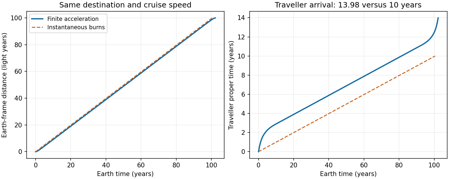
finite-acceleration correction to a relativistic cruise. Each constant-proper-acceleration leg has proper duration and Earth-frame length . ThusSubtracting the original givesFor , each accelerating leg takes about proper years and covers light years in the Earth frame, leaving positive cruise distance. The new total is about 13.98 proper years. Adding to ten years would overcount the cruise segment replaced by acceleration and braking.
Past exam of the relativity course of the University of Cambridge 2013 Paper 1 4 Solution by Codex 0 2026-10-20
Codex 0 2026-10-20redshift. An incoming radial null ray satisfies . Consecutive wave crests follow the same comoving path, so the endpoint changes in the fixed path integral obey . Comoving clocks read cosmic time; hence their measured periods and frequencies satisfyThe physical wavelength stretches with the scale factor during propagation. It is not necessary to assign a unique global inertial-frame recession velocity to a distant source.
Radial coordinate and cosmological look-back time. Differentiating gives . Combining this with the null-ray integral yieldsThe extra factor in the second denominator records the conversion from scale-factor change to elapsed cosmic time.
proper-motion distance. A small transverse displacement at emission has proper length . Define its source-frame transverse speed as ; cosmological time dilation makes . ThereforeEquivalently, , where the angular diameter distance is . The observer-time versus source-time distinction is essential. This calculation uses the stated transverse speed convention and the homogeneous background, without additional peculiar radial relativistic Doppler effect or gravitational lensing.
redshift shell volume at the present epoch. The induced spatial metric tensor on the present slice gives . Since ,This is the volume at the present epoch of the comoving shell intersected by the past light cone. Its proper volume at emission is smaller by ; a conserved population's proper number density is larger by the same factor, preserving its count.
Einstein-de Sitter cumulative number counts. In flat geometry . Inserting the stated Hubble parameter into the radial integral givesThe constant present-volume number density makes . With no members of the population before its formation epoch,As an independent check, substitution evaluates this toThis is exactly the Euclidean comoving volume per unit solid angle in the flat model. It assumes a complete count with the specified fixed population; luminosity selection, mergers or subsequent number-density evolution would require additional factors.
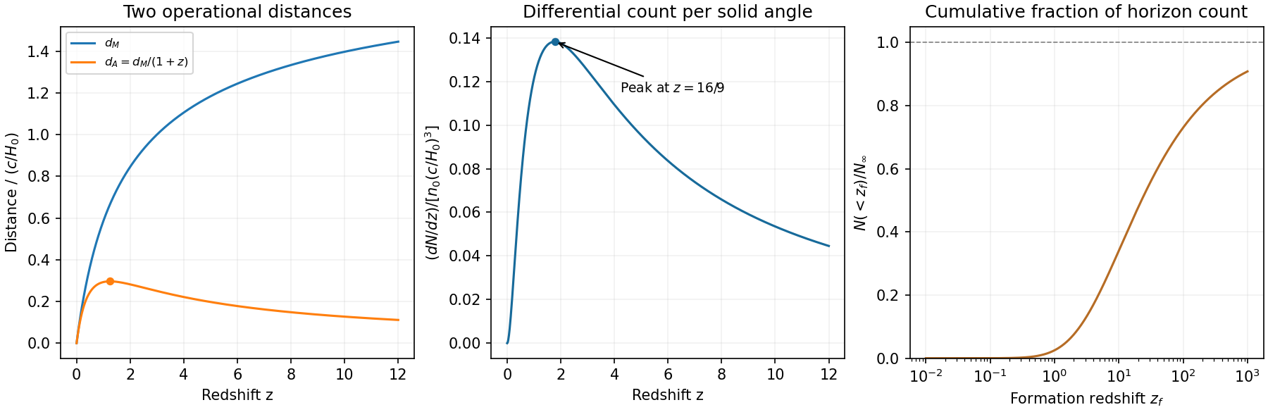
Original Einstein-de Sitter proper-motion and angular diameter distances, differential counts and cumulative fraction
. Details. Pinned article: Introduction to the OurBigBook Project
Welcome to the OurBigBook Project! Our goal is to create the perfect publishing platform for STEM subjects, and get university-level students to write the best free STEM tutorials ever.
Everyone is welcome to create an account and play with the site: ourbigbook.com/go/register. We belive that students themselves can write amazing tutorials, but teachers are welcome too. You can write about anything you want, it doesn't have to be STEM or even educational. Silly test content is very welcome and you won't be penalized in any way. Just keep it legal!
Intro to OurBigBook
. Source. We have two killer features:
- topics: topics group articles by different users with the same title, e.g. here is the topic for the "Fundamental Theorem of Calculus" ourbigbook.com/go/topic/fundamental-theorem-of-calculusArticles of different users are sorted by upvote within each article page. This feature is a bit like:
- a Wikipedia where each user can have their own version of each article
- a Q&A website like Stack Overflow, where multiple people can give their views on a given topic, and the best ones are sorted by upvote. Except you don't need to wait for someone to ask first, and any topic goes, no matter how narrow or broad
This feature makes it possible for readers to find better explanations of any topic created by other writers. And it allows writers to create an explanation in a place that readers might actually find it.
Figure 1. Screenshot of the "Derivative" topic page. View it live at: ourbigbook.com/go/topic/derivativeVideo 2. OurBigBook Web topics demo. Source. - local editing: you can store all your personal knowledge base content locally in a plaintext markup format that can be edited locally and published either:This way you can be sure that even if OurBigBook.com were to go down one day (which we have no plans to do as it is quite cheap to host!), your content will still be perfectly readable as a static site.
- to OurBigBook.com to get awesome multi-user features like topics and likes
- as HTML files to a static website, which you can host yourself for free on many external providers like GitHub Pages, and remain in full control

Figure 2. You can publish local OurBigBook lightweight markup files to either OurBigBook.com or as a static website.
Figure 3. Visual Studio Code extension installation.
Figure 5. . You can also edit articles on the Web editor without installing anything locally. Video 3. Edit locally and publish demo. Source. This shows editing OurBigBook Markup and publishing it using the Visual Studio Code extension. 
- Infinitely deep tables of contents:




All our software is open source and hosted at: github.com/ourbigbook/ourbigbook
Further documentation can be found at: docs.ourbigbook.com
Feel free to reach our to us for any help or suggestions: docs.ourbigbook.com/#contact