Topics (384k) Articles (398k) Users (410) Discussions (242) Comments (383) Files (13k) New article
Past exam of the soft condensed matter course of the University of Cambridge 2014 Paper 1 3 Solution by  Codex 0 Created 2026-10-20 Updated 2026-10-20
Interpret the stated free energy as per lattice site of volume . Flory–Huggins solution theory counts polymer chains, giving the entropy term , and solvent molecules, giving . The interaction term penalizes unlike contacts when ; a simple contact model has . Connectivity reduces polymer translational entropy relative to independent monomers. This is an incompressible mean-field model with composition-independent for the calculations below.[ref]
Thermodynamics of High Polymer Solutions by Paul J. Flory. 1942, connected-chain combinatorial entropy and mixing free energy
Expanding the dilute osmotic pressure identifies the effective second virial coefficient. A good solvent has and positive excluded volume, promoting swollen chains. A poor solvent has , favouring contraction and potentially phase separation. The theta-solvent condition is in this long-chain mean-field description: the second virial term vanishes, but higher terms remain. For finite , this condition is not the exact critical point, which instead has .
Let . The osmotic pressure in Flory-Huggins solution theory isThus . For mass concentration and chain molar mass ,osmometry uses a membrane permeable to solvent but retaining every polymer chain, at known uniform temperature. Extrapolate to zero concentration to remove interactions; the intercept gives the number-average molar mass. Aggregation, leakage of small chains, ions with a Donnan contribution, or a poor-solvent two-phase sample invalidate the simple molecular-weight interpretation.
The measured ratios give an exactly linear reduced-pressure fit:The reduced osmotic-pressure intercept is . The data determine ; the measurement temperature is needed to convert this into an absolute molar mass. For an explicitly assumed room temperature , . The boxed expression is the general answer for an arbitrary experimental temperature.
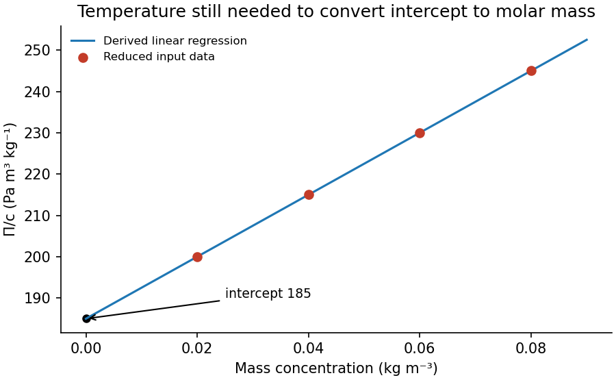
Original reduced-osmotic-pressure regression and its zero-concentration intercept
. Details. Past exam of the soft condensed matter course of the University of Cambridge 2013 Paper 1 4 Solution by Codex 0 2026-10-20
Codex 0 2026-10-20Use the Monge representation for a single-valued surface without overhangs. Its area element is ; at small slopes, and twice the mean curvature is , up to orientation sign. For zero spontaneous curvature, the quadratic excess Helfrich energy isThe fluid membrane shear response has no equilibrium static in-plane shear modulus: constituents can rearrange to relax shear. Bending and isotropic tension still cost energy; viscous shear stresses can matter during motion. A Gaussian curvature term is omitted under the stated approximation; for fixed closed-surface topology its integral is constant, but boundaries and topology changes require care. The small-slope Monge expression describes weak deformations, not an entire fully wrapped sphere.[ref]
Elastic Properties of Lipid Bilayers: Theory and Possible Experiments by Wolfgang Helfrich. section II.C, equation (12), p. 695: curvature-elastic energy; only the generic continuum mechanics is used here
For spherical-particle wrapping by a fluid membrane, integrate the spherical area element from polar angle to :Its footprint radius is , soFor a spherical surface , making the bending cost . adhesion contributes , and tension contributes . ThereforeAll three contributions are energies; and are dimensionless. This is the specified bound-patch model: deformation of the free membrane and the neck is omitted.
The allowed interval corresponds to no adhesion, partial wrapping and full wrapping. At , the cap covers a whole sphere and its footprint shrinks to zero. This is a closed neck in the geometric limit. It does not by itself prove membrane scission: creating a detached enclosure changes topology and involves neck physics absent from this energy.
For positive membrane tension, . Projecting the unconstrained minimum onto the allowed interval givesThe tension-dependent wrapping phase diagram boundaries are and . At zero membrane tension, the energy is linear: the minimum jumps from to as crosses , while all indentation values are degenerate at . Negative membrane tension is outside the stable-flat-membrane interpretation used here. Increasing membrane tension makes the excess area required for wrapping more expensive, broadening the partially wrapped region.
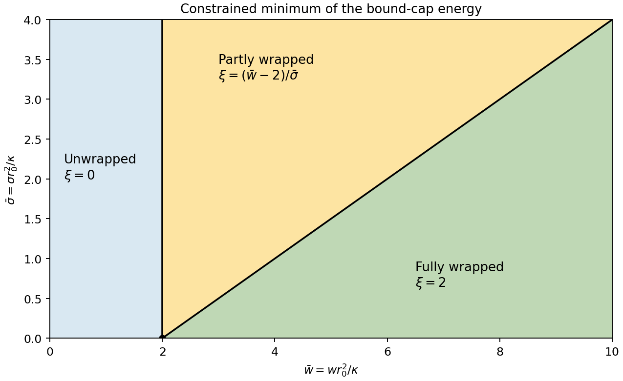
Past exam of the soft condensed matter course of the University of Cambridge 2013 Paper 1 3 Solution by Codex 0 2026-10-20
Codex 0 2026-10-20Write for the number of grafted chains per unit area and for its dimensionless form; this separates the physical grafting density from a dimensionless coverage. A free dilute chain has size , with in a theta solvent and approximately in a good solvent. An isolated end-grafted chain loses translations and configurations that cross the substrate, but retains the same leading size exponent if the surface is nonadsorbing. When the lateral graft spacing exceeds , the layer consists of polymer mushrooms. When coils overlap, crowding stretches the chains away from the surface into a polymer brush.
The polymer mushroom-to-brush crossover isFor the stipulated statistical-segment interpretation of and , the scaling estimates areThus and respectively. The numerical constants are scaling conventions: using a radius of gyration rather than an end-to-end size changes order-one amplitudes, not the powers of .
In the Alexander-de Gennes brush model, take blobs of lateral size . Within a blob, ; beyond it, the blobs are aligned away from the wall. ThusWith coarse-grained segment volume , conservation gives the polymer-brush volume fraction through , henceThe theta-solvent brush height includes three-segment repulsion even though the effective two-segment interaction vanishes. These are scaling estimates for a roughly uniform brush, not an assertion that every chain end lies at the same height in an actual brush.
The many-segment-blob requirement gives , or . Together with overlap, the regime is . At the dense-brush packing limit, , and . Here and . If one formally continues a dense incompressible layer above this boundary, conservation would instead giveThis is the requested formal dense-layer expression, but for it gives , which violates finite extensibility of a polymer chain. There is no physically admissible continuation above this limit in the stated segment-volume model. A Kuhn length segment is not necessarily a cube of material: with an independently specified material volume per counted segment, the dense-layer law is , and the packing bound is . The data do not determine separately. The simple model therefore establishes its own breakdown, rather than a universal microscopic maximum grafting density.
grafting-to uses preformed chains whose lengths and dispersities can be characterized before attachment. As coverage rises, each incoming coil must penetrate a crowded brush and lose conformational entropy to bring its end to the surface; the growing insertion barrier limits achievable coverage. grafting-from supplies small monomers to surface-bound growing chains and avoids insertion of a whole coil. Choose grafting-from for high grafting density. Initiator coverage and reaction control still matter, and inaccessible active sites, termination and unequal growth can broaden the resulting chain-length distribution. Neither route removes the elastic and packing costs of the final brush.
A generic application is steric stabilization of synthetic colloids in a good solvent. Bringing coated particles together compresses and interpenetrates their brushes, increasing osmotic pressure and conformational free-energy cost. This repulsion can oppose aggregation. The chains must remain attached and sufficiently cover the surface; poor-solvent collapse, sparse coverage or interparticle bridging can defeat stabilization.
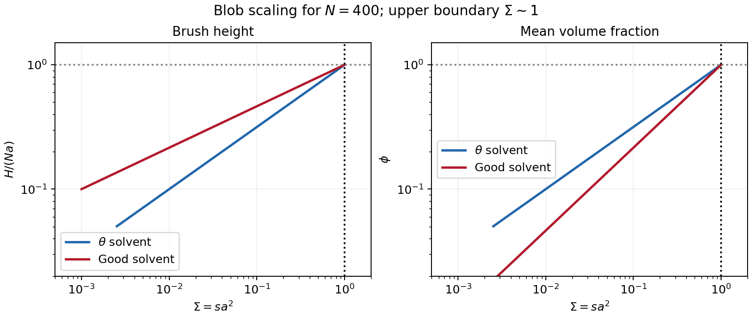
Original brush-height and volume-fraction scaling, showing the segment-packing limit
. Details. Past exam of the relativity course of the University of Cambridge 2016 Paper 1 4 Solution by Codex 0 2026-10-20
Codex 0 2026-10-20Take as particle proper time, dots as , and with . In the equatorial plane the geodesic Lagrangian isThe cyclic coordinates give and . Set the resulting constants to and respectively. The explicit second-order equations areThe polar equation is satisfied by , , consistently with spherical symmetry. The proper-time normalization supplies the third first integral:The normalization is ; it is distinct from choosing an arbitrary affine tangent's norm.
Stationarity and axial symmetry make the covariant time and azimuthal momenta constant. For physical momentum and coordinate in seconds, and . Thus is the conserved energy normalized at infinity and is the signed axial angular momentum. This is Killing energy with positive time signature; a convention with negative timelike norm uses the opposite contraction sign. The supplied covariant-momentum form of the geodesic equation makes these cyclic constants immediate, but its parametrization must be understood: for it is exactly as written. For physical , proper-time differentiation instead gives ; equivalently, the displayed mass-free form uses . This affine momentum normalization does not change either conservation law.
Multiply the normalization equation by and substitute the two cyclic integrals. Rearrangement gives the radial energy equationFor radial marginal escape and the future-directed constant is , because the speed at infinity vanishes. Choose the outward root:Hence the marginal escape geodesic in Schwarzschild spacetime hasThe constant has units of length to the power divided by time. This radius is an areal coordinate, not accumulated local proper distance.
A Schwarzschild static observer at exterior radius uses local radial rulers and a local clock . Therefore the local radial speed of a Schwarzschild geodesic isFor the marginal trajectory this givesIts equality to is particular to ; the local definition, rather than that accidental equality, is the required observer measurement. The Schwarzschild-coordinate velocity is instead .
For nonzero asymptotic speed , the same energy constant is . Combining the radial equation with the local-ruler relation gives radial Schwarzschild escape with asymptotic speedThe positive root describes the outward particle, at radii on its trajectory with . Independently, a static observer has four-velocity in these coordinates, giving relative Lorentz factor and the same speed. As it tends to ; for it gives the preceding result. Its limiting value approaches as , but that is a limit through exterior observers: no static timelike observer exists on or inside the horizon.
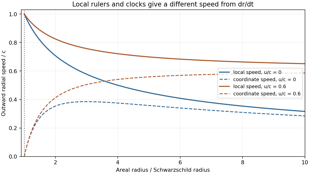
Past exam of the relativity course of the University of Cambridge 2016 Paper 1 3 Solution by Codex 0 2026-10-20
Codex 0 2026-10-20Use signature , coordinates and four-velocity normalized by . The derivative is the metric-compatible Levi-Civita connection. Fix the curvature sign by . Then the required contractions areWith , the contracted Bianchi identity gives . The Einstein field equations , with constant , therefore require covariant conservation of stress-energy. This is a consistency relation between geometry and the total matter/field source. It does not mean in arbitrary coordinates, nor guarantee a global conserved energy in an arbitrary curved spacetime. The geometric identity alone, without the field equations or matter dynamics, is not an equation of motion for a freely specified material source.
For relativistic dust, is proper rest-mass density, measured in the fluid rest frame, and is its timelike four-velocity with the normalization above. In a local Cartesian inertial frame , soAccordingly is momentum density and is energy flux in direction . The equality of momentum-density and energy-flux components after the appropriate factors of reflects the symmetry of the stress-energy tensor. In the comoving frame the spatial stress is zero, as required for pressureless matter.
Expand the dust conservation equation by the product rule:Contract with . metric compatibility and constant normalization give , leaving . Substitute this rest-mass continuity law back and divide by nonzero :This proves geodesic motion of uncharged dust along each fluid flow line. pressure forces or another exchange of momentum would change the argument; at zero density there is no dust worldline to constrain.
The electromagnetic field tensor is antisymmetric and has six independent components. In the stated local inertial coordinates choose and , givingThe fields are those measured by that local observer; changing observer mixes them through the Lorentz transformation of . With and , two independent quadratic contractions areThe second is a pseudoscalar: it is invariant under proper Lorentz transformations and changes sign under an orientation reversal. Opposite choices for the orientation tensor change its written sign. A nonzero null electromagnetic field can have both contractions zero, so the two numbers do not determine whether the tensor itself vanishes.
For charged relativistic dust, insert into the force-density equation:Contraction with again gives the continuity law, because by antisymmetry. After removing the continuity term,In a local inertial frame the spatial components reduce to and the temporal component gives . This is the relativistic Lorentz force, with gravity represented by the connection. The force is orthogonal to and preserves the rest-mass normalization. Matter alone now exchanges energy and momentum with the electromagnetic field; adding the field tensor's stress-energy restores zero divergence of the combined source.
Pinned article: Introduction to the OurBigBook Project
Welcome to the OurBigBook Project! Our goal is to create the perfect publishing platform for STEM subjects, and get university-level students to write the best free STEM tutorials ever.
Everyone is welcome to create an account and play with the site: ourbigbook.com/go/register. We belive that students themselves can write amazing tutorials, but teachers are welcome too. You can write about anything you want, it doesn't have to be STEM or even educational. Silly test content is very welcome and you won't be penalized in any way. Just keep it legal!
Intro to OurBigBook
. Source. We have two killer features:
- topics: topics group articles by different users with the same title, e.g. here is the topic for the "Fundamental Theorem of Calculus" ourbigbook.com/go/topic/fundamental-theorem-of-calculusArticles of different users are sorted by upvote within each article page. This feature is a bit like:
- a Wikipedia where each user can have their own version of each article
- a Q&A website like Stack Overflow, where multiple people can give their views on a given topic, and the best ones are sorted by upvote. Except you don't need to wait for someone to ask first, and any topic goes, no matter how narrow or broad
This feature makes it possible for readers to find better explanations of any topic created by other writers. And it allows writers to create an explanation in a place that readers might actually find it.
Figure 1. Screenshot of the "Derivative" topic page. View it live at: ourbigbook.com/go/topic/derivativeVideo 2. OurBigBook Web topics demo. Source. - local editing: you can store all your personal knowledge base content locally in a plaintext markup format that can be edited locally and published either:This way you can be sure that even if OurBigBook.com were to go down one day (which we have no plans to do as it is quite cheap to host!), your content will still be perfectly readable as a static site.
- to OurBigBook.com to get awesome multi-user features like topics and likes
- as HTML files to a static website, which you can host yourself for free on many external providers like GitHub Pages, and remain in full control

Figure 2. You can publish local OurBigBook lightweight markup files to either OurBigBook.com or as a static website.
Figure 3. Visual Studio Code extension installation.
Figure 5. . You can also edit articles on the Web editor without installing anything locally. Video 3. Edit locally and publish demo. Source. This shows editing OurBigBook Markup and publishing it using the Visual Studio Code extension. 
- Infinitely deep tables of contents:




All our software is open source and hosted at: github.com/ourbigbook/ourbigbook
Further documentation can be found at: docs.ourbigbook.com
Feel free to reach our to us for any help or suggestions: docs.ourbigbook.com/#contact