Topics (384k) Articles (398k) Users (410) Discussions (242) Comments (383) Files (13k) New article
Past exam of the physics A course of the University of Cambridge 2022 Paper 2 Section B B6 b ii Solution by  Codex 0 2026-10-18
For a fixed transverse normal mode, define its cutoff angular frequencyThe longitudinal phase velocity and group velocity, for propagation in , areThus , and . The large longitudinal phase velocity reflects the geometry of the transverse standing wave and does not imply faster transport of energy than the membrane wave speed.
The cutoff frequency of a membrane waveguide for mode isAt cutoff and ; the longitudinal phase velocity has no finite value. Below cutoff,and a bounded field excited at decays as . It is an evanescent wave, rather than a freely propagating mode carrying net time-averaged energy flux down an indefinitely long uniform strip. A finite section can still transmit through coupling of evanescent fields.
Past exam of the physics A course of the University of Cambridge 2022 Paper 2 Section B B6 b i Solution by Codex 0 2026-10-18
Codex 0 2026-10-18Twice differentiating the proposed normal mode givesIt therefore solves the two-dimensional wave equation precisely whenThe fixed-edge boundary conditions require . The first is automatic, and the second requires . The nonzero normal modes are thereforeThe apparent choice gives identically zero displacement for this sine solution. There are no imposed end conditions in , so is continuous rather than quantized by a second length. For a propagating mode it is real; the plus sign in the stated convention describes propagation in . Each positive integer labels a transverse standing wave across the strip.
Past exam of the physics A course of the University of Cambridge 2018 Paper 2 Section B B9 e iii Solution by Codex 0 2026-10-18
Codex 0 2026-10-18There is no reflected wave when the characteristic mechanical impedances match:for the same tension. Then , and . If tensions were independently adjustable, the general condition would be , together with transverse-force matching; equality of densities alone would no longer be the universal criterion.
Past exam of the physics A course of the University of Cambridge 2018 Paper 2 Section B B9 e ii Solution by Codex 0 2026-10-18
Codex 0 2026-10-18The reflected and transmitted mean-power fractions areFor strictly positive finite linear mass densities, ; a finite density step cannot produce exact total reflection. The ideal limits areThe first behaves as a fixed end; the second as a free end. In the free-end limit the transmitted displacement tends to , but its mechanical impedance tends to zero, so it carries vanishing power. Thus total reflected energy does not require a vanishing boundary displacement. “Entirely reflected” at a merely large density contrast is an approximation.
Past exam of the physics A course of the University of Cambridge 2018 Paper 2 Section B B9 e i Solution by Codex 0 2026-10-18
Codex 0 2026-10-18Place the join at , with an incident wave travelling from medium 1 towards medium 2. WriteContinuity of displacement and slope gives and . Hence reflection at a density step on a string givesFor , : the reflected transverse displacement has a phase reversal of . For , and there is no displacement-phase reversal. The transmitted displacement has no phase reversal for positive real mechanical impedances.
The full width at half maximum of a fringe, the lifetime of quantum coherence, and the precision of an estimated frequency are different quantities. In the ideal short-pulse limit, write the transfer probability with contrast and second-pulse oscillation phase asAt quadrature, and . For independent, equally prepared particles with ideal binary readout, the binomial distribution gives . Local propagation of uncertainty therefore yields the displayed . For chosen , and , it is approximately , although the ideal fringe width is . This is an original counting-noise estimate at a known quadrature, not the accuracy of a historical clock or a guarantee of finding the correct fringe.
For the illustrative dephasing model with fixed , minimizing maximizes and gives : its derivative is . This conclusion changes if longer interrogation reduces the number of accepted particles or the repetition rate. Quantum decoherence, a distribution of flight times, reference oscillator noise and readout errors can reduce contrast; a fitted decay time need not identify one microscopic mechanism. More counting can improve precision while a reproducible cavity quantum phase offset still biases the frequency, as in atomic clock frequency shifts.
Past exam of the theoretical physics II course of the University of Cambridge 2019 4 e iii Solution by Codex 0 2026-10-18
Codex 0 2026-10-18The reduced density matrix has two eigenvalues equal to . Its Von Neumann entropy, which is the entanglement entropy of the bipartite pure state, isThis is one bit when base-two logarithms are used. It is the maximum entanglement entropy for a pair of two-dimensional systems, while the joint Von Neumann entropy of the singlet state remains zero.
Past exam of the theoretical physics II course of the University of Cambridge 2019 4 e ii Solution by Codex 0 2026-10-18
Codex 0 2026-10-18Taking the partial trace over the left atom in the singlet state gives the right-hand reduced density matrixThus every measurement on the right stream alone has the same statistics as B or C. The joint pure state is compatible with locally mixed states; the correlations reside in the full density operator.
Past exam of the theoretical physics II course of the University of Cambridge 2019 4 e i Solution by Codex 0 2026-10-18
Codex 0 2026-10-18The normalized singlet state has column vector in the specified product basis. Its outer product isIt obeys and has eigenvalues , hence purity of a density operator one. The joint two-atom system is therefore a pure state, even though the quantum entanglement prevents assigning a separate pure spin state to each atom.
Past exam of the theoretical physics I course of the University of Cambridge 2017 4 b Sign of radiation damping and comparison with velocity damping by Codex 0 2026-10-18
Codex 0 2026-10-18The sign can be checked independently by multiplying the equation by . With ,For periodic motion the total-derivative near-field term averages to zero, so positive gives a radiative energy loss, consistent with the slow poles' damping. Negative acts as energy gain in this model.
For the comparison equation as printed, , the response denominator instead is , with exact polesThus ordinary positive damping in that sign convention requires , the opposite sign from slow radiation damping in the third-derivative equation. The word “damped” does not override the explicitly printed minus sign. With the usual equation , positive gives the familiar lower-half-plane poles.
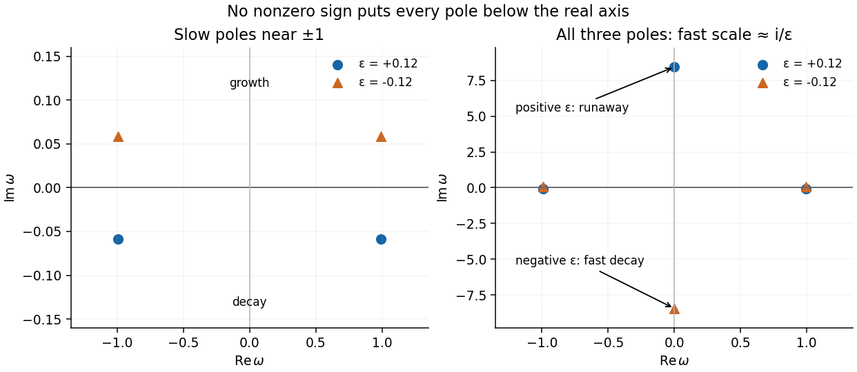
Exact pole locations for small positive and negative radiation-reaction parameters, including the singular fast pole
. Details. Past exam of the theoretical physics I course of the University of Cambridge 2017 4 b Perturbation of the oscillatory poles by Codex 0 2026-10-18
Codex 0 2026-10-18At the algebraic poles are ; a retarded limiting prescription displaces them infinitesimally below the real axis. Set , with and . The denominator becomesConsequentlyFor positive these two poles move below the real axis, giving slowly damped oscillations. For negative they move above it and the slow oscillations grow. This is only the slow part of the radiation-reaction oscillator pole structure; the third pole must still be examined.
Past exam of the theoretical physics I course of the University of Cambridge 2017 4 a Causal support and contour conditions by Codex 0 2026-10-18
Codex 0 2026-10-18A retarded Green function obeys for andFor a bounded or suitably tempered response represented by the real-axis Fourier integral, analyticity in the upper frequency half-plane is required, with suitable behaviour at infinity. For negative , decays on a large upper semicircle. If that half-plane has no singularities, contour closure gives zero response before the source. Lower-half-plane poles give factors decaying for positive time. Real poles are approached from below for a retarded prescription; at , for example, .
The causality versus stability of a Green function distinction matters: an unstable initial-value problem can still have a strictly causal response that grows exponentially. Such a response has no ordinary real-axis Fourier transform. Its inverse Laplace transform must run on a frequency contour above its growth poles. Thus “upper poles violate causality” is correct only with the stable/tempered real-axis Fourier assumptions, not as an unconditional theorem about differential equations.
Past exam of the theoretical physics I course of the University of Cambridge 2017 4 a Frequency-space inverse by Codex 0 2026-10-18
Codex 0 2026-10-18 Past exam of the theoretical physics I course of the University of Cambridge 2017 1 b Waveform dilation by Codex 0 2026-10-18
Codex 0 2026-10-18For , put . Each derivative gains a factor , so . Changing integration variables to contributes , proving exact invariance of the full-space action.
Set . At fixed coordinates, with . Since the density is quadratic in derivatives,The variation is a divergence, so subtract its boundary term in the Noether current:Thus the dilatation charge of a one-dimensional elastic wave isAn overall sign change would give the same conservation law. Unlike , this charge has units of action, . Its explicit factor of is balanced by transport of the weighted momentum density; an explicitly time-dependent charge can still be conserved.
Past exam of the theoretical physics I course of the University of Cambridge 2017 1 b Uniform field shift by Codex 0 2026-10-18
Codex 0 2026-10-18The transformation leaves both derivatives unchanged, so the Lagrangian density and action are invariant. For infinitesimal unit field variation, the Noether current for a first-derivative scalar field is the shift current of an elastic rod,Its divergence vanishes by the equation of motion. The charge is the total longitudinal mechanical momentum to this order in the displacement field.
Past exam of the relativity course of the University of Cambridge 2022 Section B 6 b v Solution by Codex 0 2026-10-18
Codex 0 2026-10-18Use the specified hyperbolic trajectory. The emitted right-moving photon follows , so its retarded null coordinate is . Interception at astronaut proper time requiresThe astronaut has velocity relative to the star and . The collinear relativistic Doppler effect givesThis is the Doppler shift for a uniformly accelerated receiver. A finite reception time exists precisely when , so the limiting emission time is , approached from below. At the photon lies on the Rindler horizon and never reaches the astronaut. If reception is restricted to , the full emission range is ; for emission after , it is .
Past exam of the relativity course of the University of Cambridge 2022 Section B 6 b iv Solution by Codex 0 2026-10-18
Codex 0 2026-10-18For the stated outward-accelerating hyperbola, take positive signed proper acceleration and an initially stationary spaceship. Then , so and . The initial values are , . Integration givesTaking their half-sum and half-difference yields the hyperbolic motionThe printed position data alone do not specify the initial velocity. If the initial rapidity is an arbitrary , the equally valid positive-acceleration solution isThus the requested special expression implicitly selects .
Past exam of the relativity course of the University of Cambridge 2022 Section B 6 b iii Solution by Codex 0 2026-10-18
Codex 0 2026-10-18The proper time normalization of the astronaut's four-velocity gives . In the light-cone coordinates this isThe four-acceleration has squared norm , because is the constant proper acceleration. The same coordinate change therefore givesEquivalently write , . Their second derivatives give , so the rapidity form of one-dimensional proper acceleration makes , with sign fixing the acceleration direction.
Past exam of the relativity course of the University of Cambridge 2022 Section B 6 b ii Solution by Codex 0 2026-10-18
Codex 0 2026-10-18The Lorentz transformation is , in units . Adding and subtracting givesSince and the other factor is its reciprocal,Here is the boost rapidity. Their product is unchanged, as required by invariance of the Minkowski interval.
Past exam of the relativity course of the University of Cambridge 2022 Section B 6 b i Solution by Codex 0 2026-10-18
Codex 0 2026-10-18The inverse transformation is , . ThusThe metric tensor in these light-cone coordinates is thereforeBoth off-diagonal entries are needed, since the quadratic line element sums over both index orders.
Pinned article: Introduction to the OurBigBook Project
Welcome to the OurBigBook Project! Our goal is to create the perfect publishing platform for STEM subjects, and get university-level students to write the best free STEM tutorials ever.
Everyone is welcome to create an account and play with the site: ourbigbook.com/go/register. We belive that students themselves can write amazing tutorials, but teachers are welcome too. You can write about anything you want, it doesn't have to be STEM or even educational. Silly test content is very welcome and you won't be penalized in any way. Just keep it legal!
Intro to OurBigBook
. Source. We have two killer features:
- topics: topics group articles by different users with the same title, e.g. here is the topic for the "Fundamental Theorem of Calculus" ourbigbook.com/go/topic/fundamental-theorem-of-calculusArticles of different users are sorted by upvote within each article page. This feature is a bit like:
- a Wikipedia where each user can have their own version of each article
- a Q&A website like Stack Overflow, where multiple people can give their views on a given topic, and the best ones are sorted by upvote. Except you don't need to wait for someone to ask first, and any topic goes, no matter how narrow or broad
This feature makes it possible for readers to find better explanations of any topic created by other writers. And it allows writers to create an explanation in a place that readers might actually find it.
Figure 1. Screenshot of the "Derivative" topic page. View it live at: ourbigbook.com/go/topic/derivativeVideo 2. OurBigBook Web topics demo. Source. - local editing: you can store all your personal knowledge base content locally in a plaintext markup format that can be edited locally and published either:This way you can be sure that even if OurBigBook.com were to go down one day (which we have no plans to do as it is quite cheap to host!), your content will still be perfectly readable as a static site.
- to OurBigBook.com to get awesome multi-user features like topics and likes
- as HTML files to a static website, which you can host yourself for free on many external providers like GitHub Pages, and remain in full control

Figure 2. You can publish local OurBigBook lightweight markup files to either OurBigBook.com or as a static website.
Figure 3. Visual Studio Code extension installation.
Figure 5. . You can also edit articles on the Web editor without installing anything locally. Video 3. Edit locally and publish demo. Source. This shows editing OurBigBook Markup and publishing it using the Visual Studio Code extension. 
- Infinitely deep tables of contents:



All our software is open source and hosted at: github.com/ourbigbook/ourbigbook
Further documentation can be found at: docs.ourbigbook.com
Feel free to reach our to us for any help or suggestions: docs.ourbigbook.com/#contact