Topics (374k) Articles (387k) Users (410) Discussions (242) Comments (383) Files (13k) New article
In a flexible crosslinked polymer network, deformation restricts the configurations of chain segments between cross-links. The resulting decrease of entropy produces a restoring entropic force. For an ideal affine Gaussian network, the shear modulus is , where is the number density of elastically active strands. A nearly incompressible isotropic rubber has Young's modulus . At fixed network density within the rubbery regime, both increase approximately linearly with absolute temperature. This statement does not describe crossing the glass transition or chemical degradation.
A rubbery material based mainly on cis-rich polyisoprene. A lightly crosslinked network provides recoverable deformation through rubber elasticity.
Einstein's Miraculous Year On a Heuristic Point of View Concerning the Production and Transformation of Light by Albert Einstein by  Codex 0 2026-10-18
Cited passages: §§7–8, pp. 191–196.
UNSW School of Physics documents a Doppler effect experiment using a buzzer based on piezoelectricity, powered by a taped-on battery, and a computer's built-in microphone. Audacity records the acoustic wave. First record the stationary source to establish its baseline frequency; then attach it to a bicycle passing the stationary microphone. The published spectrogram shows a rapid decrease in frequency during passage.[ref]
Measuring velocities using the Doppler Shift at UNSW School of Physics. UNSW, Measuring velocities using the Doppler Shift: Introduction, Figs. 1–2; Circular Motion, Measurements (2)–(3); Linear Motion:Bicycle, Moving Source
For numerical readout, select an approaching or receding interval, display its frequency spectrum using Plot Spectrum, and read the interpolated Peak frequency. The protocol recommends repeating with slightly different selections to test stability, and working outdoors to reduce reflections and standing waves. Longer windows refine frequency spacing while averaging over more motion. The baseline controls for the source's actual tone; repeated selections expose analysis-window sensitivity.[ref]
Measuring velocities using the Doppler Shift at UNSW School of Physics. UNSW, Introduction, final paragraph; Circular Motion, spectrogram resolution discussion; Linear Motion:Bicycle, Plot Spectrum and Peak instructions
Under nearly collinear constant-speed approach, infer from the classical Doppler effect for sound. For recession the positive speed is . These inversions need a specified speed of sound. An offset path changes the projection, as in Doppler frequency along a trajectory; neither inversion measures the full speed near closest passage. The protocol's controls cannot remove arbitrary acceleration, background measurement noise or unresolved reflected paths. No new measurements are claimed here.
In the same uniform stationary sound model, let be emission time, reception time, and and source and receiver positions. The direct-path propagation condition and its direction areThe unit vector points from the source's old emission position to the receiver's reception position. With velocities and , taking a derivative of the propagation condition givesHere the dot products project onto the actual propagation direction. The last equality counts source wave phase cycles at reception for constant emitted frequency . It assumes both speeds are below , a unique direct arrival and smooth motion; interpreting a measured short-window frequency spectrum additionally requires little frequency change within that window. The source velocity must be evaluated at emission, not at reception. This delayed geometry matters when the direction changes.
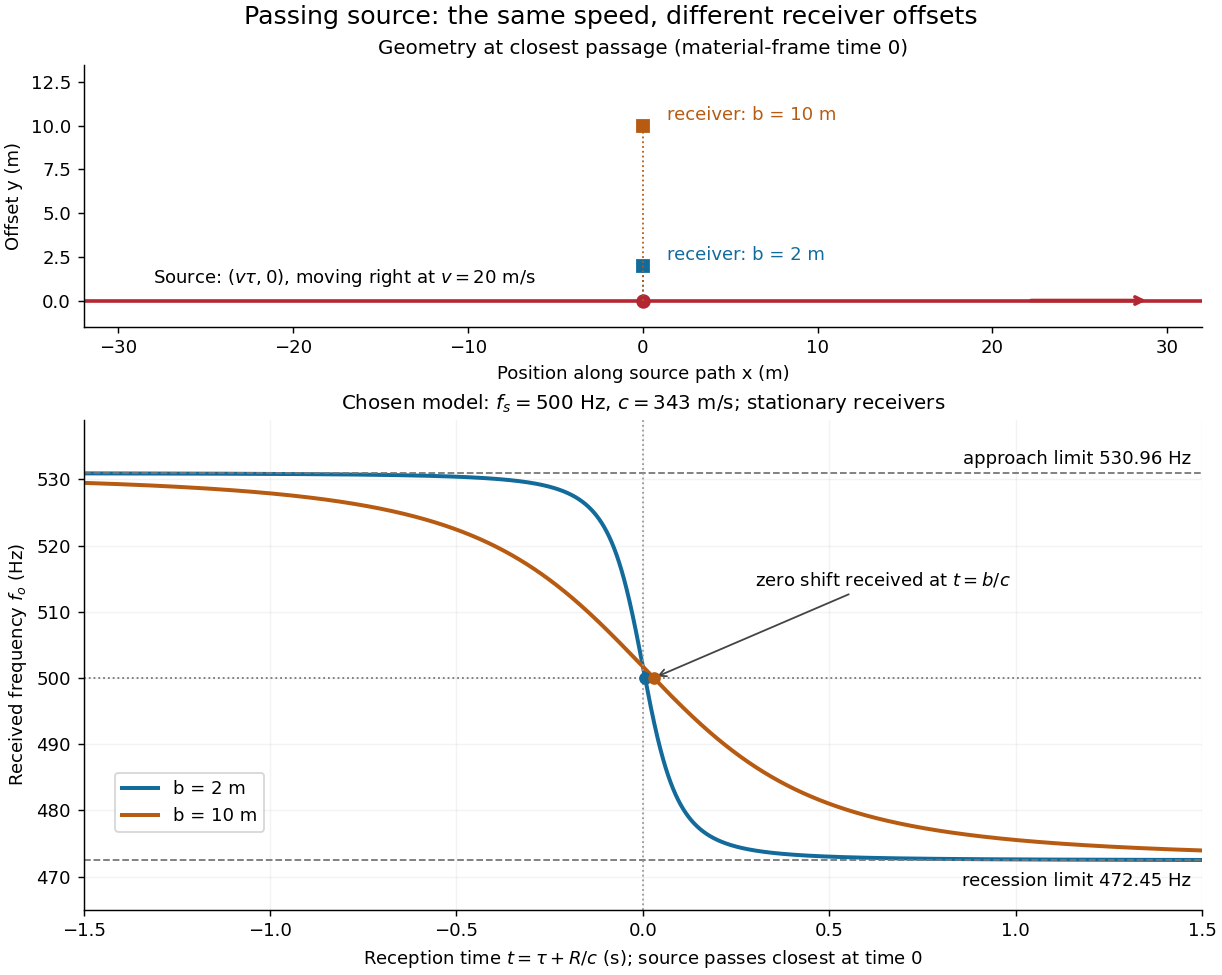
For an original pass-by model, a source follows and a stationary receiver is at with . The source passes its closest position at emission time . ThenThese parametric equations give received frequency against reception time. For the shift is positive, for negative, and the unshifted emission at reaches the receiver at . Thus zero shift occurs after the source's geometric closest passage in the material's reference frame. Increasing spreads the transition over a longer interval even though is unchanged. Far before and after passage, the frequency approaches and respectively.
Work in the material's rest reference frame, with constant speed of sound . For one-dimensional propagation, choose the positive direction along the travelling wave from its emission point toward the receiver. Define and as the signed source and receiver velocities along that same axis. Both use the same sign convention: positive moves the source toward the receiver ahead, whereas positive moves that receiver away from the incoming wave. Assume and , constant velocities, and no source-receiver crossing during the interval considered. Then
To derive this, let be the emission wave period. During , one wave crest travels while the source advances . Successive wavefronts along the chosen direction therefore have wavelengthThey overtake the receiver at relative speed , so counting wave crests gives . This separates the source's effect on wavelength from the receiver's effect on crossing rate. Even with a moving source, a stationary receiver obeys because the wave speed through the material remains .
For a stationary receiver and a source approaching at speed , set and : . For recession choose the positive axis along the departing wave toward the receiver again, so the source has : . For the deliberately chosen values , and , the two predictions areThe corresponding wavelengths are and , compared with for a stationary source. These are calculations for chosen parameters, not reported measurements.
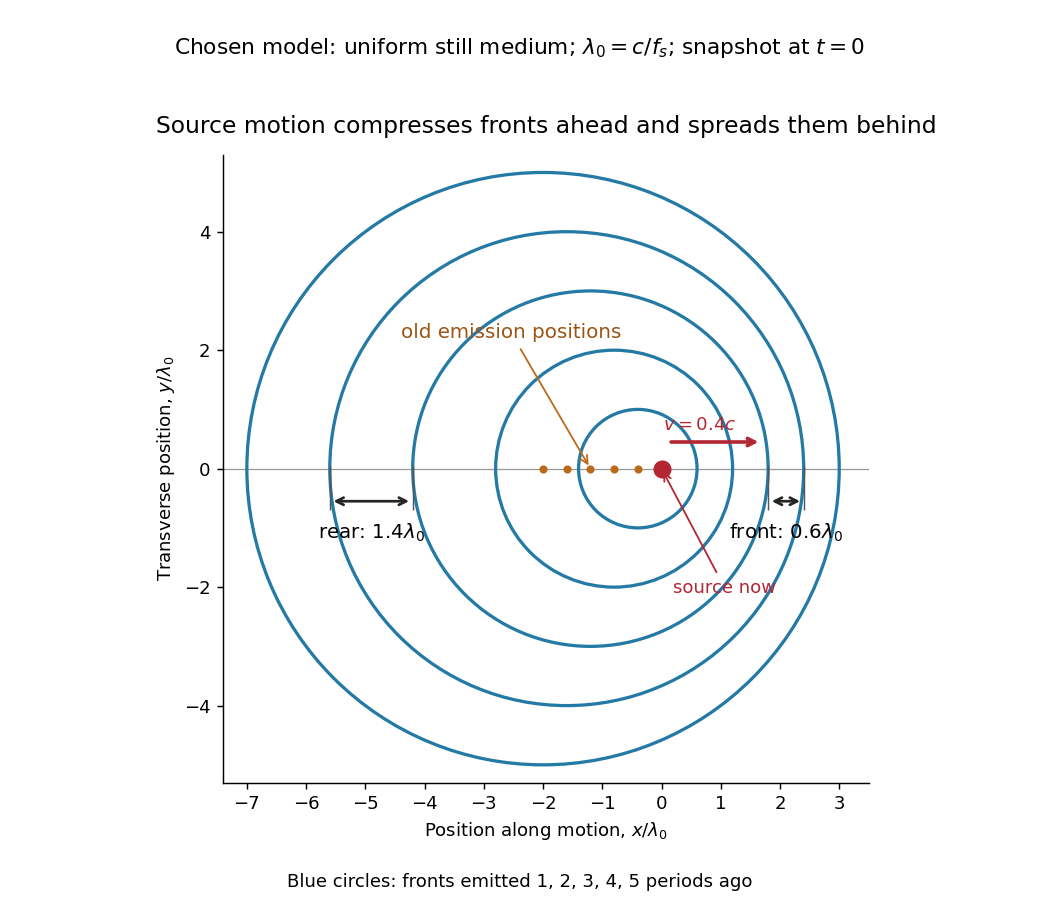
Moving-source wavefront spacing in the classical Doppler effect for sound
. Original linear acoustics model at , with a deliberately enlarged speed ratio for readability. Lengths are measured in . Successive circles are sections of spherical wavefronts emitted one wave period apart; their centres stay at the old emission positions. The forward spacing is and the rear spacing . These chosen parameters differ from the worked example. Details.A receiver approaching a stationary source at instead has , , giving . Moving away gives . The equal closing speeds do not make these equal to the moving-source values. If both source and receiver move together with , however, the numerator and denominator cancel and . For speeds small compared with , the first-order shift is ; the difference between moving-source and moving-receiver experiments appears beyond this first order.
A shallow donor impurity in an isotropic semiconductor can be approximated by an electron of effective mass in a Coulomb potential screened by relative permittivity . Its ground-state binding energy and radius areThe donor level lies below the conduction band. These are magnitudes: the bound electron's energy relative to the band edge is negative. Band anisotropy, short-distance impurity structure and screening by mobile carriers can invalidate the simple Bohr model rescaling.
For shallow hydrogenic donor states of radius and random donor number density , the mean spacing is of order . Taking this spacing comparable to gives ; a geometric diameter criterion instead gives . The orbitals have exponentially decaying tails rather than hard boundaries, so there is no exact geometric onset. Appreciable overlap also limits the independent-donor ionisation model; a genuine transport transition needs additional electronic physics.
Splitting two integers in positional notation gives and , where shifts a block by numeral digits in fixed radix . The distributive property givesComputing separately needs four block multiplications. Merely halving the operands therefore gives an ideal recurrence relation , still with quadratic time complexity. The Karatsuba three-product identity instead computes , and , recovering the middle coefficient by two subtractions. The MIT notes present precisely this four-product versus three-product distinction.[ref]
Lecture 11: Numerics I. 6.006 Introduction to Algorithms, Fall 2011, Lecture 11: Numerics I, printed pp. 4–5, High Precision Multiplication and Karatsuba's Method
For an original small example, multiply by . Set , , , , . Four separate block products would give , , , . The three-product calculation isThe crucial reuse is that and supply the outer coefficients and also remove the unwanted terms from . There is no need to compute and separately. Expanding proves the identity. Induction extends it to Karatsuba multiplication once each smaller block product is correct and Karatsuba recursion termination supplies decreasing sizes and complete base cases.
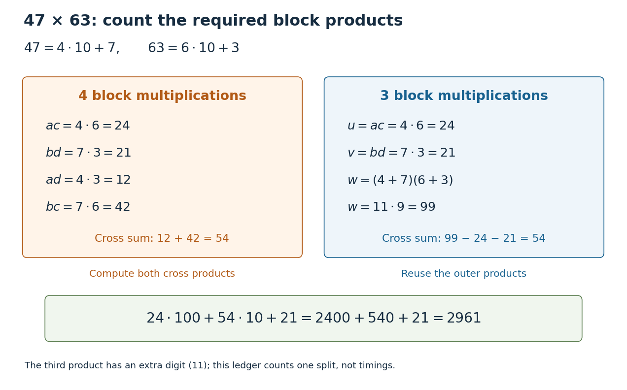
Four block products or three: the exact ledger for
. The left ledger computes both cross products separately. The right ledger reuses and to recover their sum as . Both reconstructions yield . Counts refer to block multiplication calls at this split; the extra numeral digit in prevents interpreting all three as single-digit products. Details.The operation model matters. Let count numeral digits in fixed radix , and count single-digit multiplication, addition, subtraction and copying as constant-cost operations. The nonrecursive work on size- operands is : it includes forming sums, positional shifts and Karatsuba carry handling. Treating an arbitrarily large integer multiplication as one operation would hide the very saving being studied. The coefficients above must be shifted and added; concatenating them does not give .
In the ideal equal-half model, Karatsuba multiplication has . At depth its additional work is at most a constant times , and its leaf count is for . A geometric series gives , where . Four recursive products would instead give leaves. Saving one block product repeatedly changes the exponent, even though the combination requires extra addition and subtraction.
For the literal sum-based version, each operand sum can occupy one extra numeral digit. Its worst-case upper recurrence relation is for a nondecreasing cost envelope, above a fixed base case threshold of at least three digits. Karatsuba digit-operation cost proves that this extra digit preserves the exponent; Karatsuba operand splitting handles odd lengths and leading zero padding. For signed integers, apply the nonnegative procedure to their absolute values and restore the sign. The small ledger establishes an exact identity, while Karatsuba practical crossover explains why it alone cannot predict a speedup for two-digit operands.
The combination cost is the work needed to reconstruct an answer from the returned smaller answers. In a time complexity calculation, also count partitioning the input, preparing arguments, and other work outside recursive calls. Write their total as for a size- call. For an ideal balanced divide-and-conquer algorithm making calls of size , the recurrence relation iswhere is a fixed positive integer and is the base case cost. Take , a power of two, so the size becomes one after exactly divisions. This is a model of total sequential work: all smaller calls contribute, even if a machine could run some simultaneously.
At level , there are calls, each of size . Expanding the recurrence relation gives the exact identityThe first term counts the base cases; the sum stops before their level because describes work in nonterminal calls. This separates depth, number of calls, and local work. Merge sort has two smaller calls and a linear merge algorithm, giving in Big O notation. The MIT notes derive this by summing equal work across levels, and contrast it with the same two-way split followed by quadratic local work.[ref]
Lecture 3: Insertion sort, merge sort. 6.006 Introduction to Algorithms, Fall 2011, Lecture 3: slides 32–44, recurrence and equal work per level; slide 46, quadratic local work
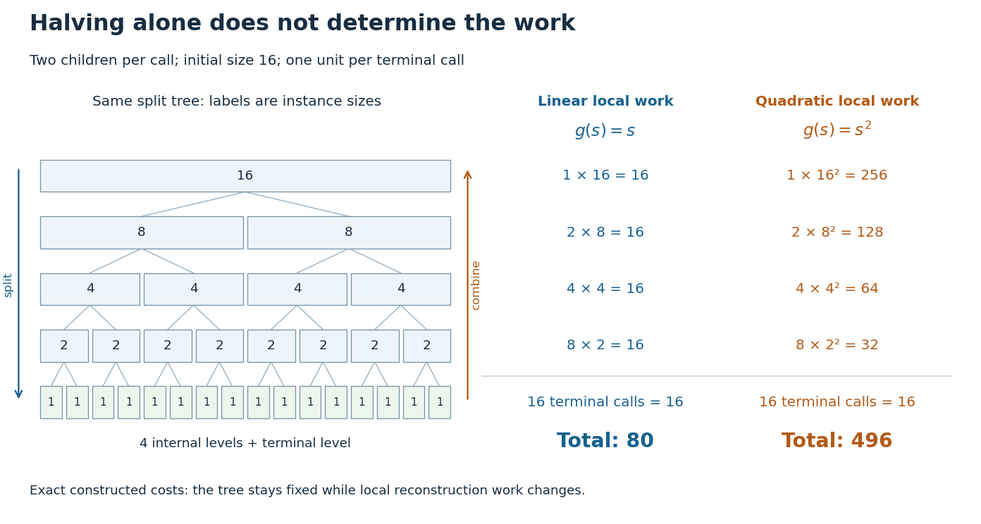
The same halving tree can have linear or quadratic work at each call
. Original exact cost models with , two children per nonterminal call, and one unit per base case. For local work , every internal level costs 16 and the total is 80. For , internal levels cost 256, 128, 64, 32 and the total is 496. The tree shows instance sizes; the ledger counts work rather than execution order. Details.For the first constructed model, set , and . Every internal level costs , while the leaves cost . Thus , giving . If the same split instead has , then the finite geometric series givesso . The root alone already costs in this second model. Smaller arguments do not eliminate expensive reconstruction. These are stipulated operation counts, rather than measured running times or exact merge sort instruction counts.
Binary search has a different saving: after its comparison, only one half remains a candidate. With constant-cost indexed array access and comparisons, its worst-case time complexity satisfies an upper recurrence relation for , with . There is one continuing branch, rather than two. At most nonempty candidate ranges are inspected for . Copying the retained half into a fresh array on every step would add linear work at that step and lose this logarithmic bound. The shrinking range and its representation both matter.
Pinned article: Introduction to the OurBigBook Project
Welcome to the OurBigBook Project! Our goal is to create the perfect publishing platform for STEM subjects, and get university-level students to write the best free STEM tutorials ever.
Everyone is welcome to create an account and play with the site: ourbigbook.com/go/register. We belive that students themselves can write amazing tutorials, but teachers are welcome too. You can write about anything you want, it doesn't have to be STEM or even educational. Silly test content is very welcome and you won't be penalized in any way. Just keep it legal!
Intro to OurBigBook
. Source. We have two killer features:
- topics: topics group articles by different users with the same title, e.g. here is the topic for the "Fundamental Theorem of Calculus" ourbigbook.com/go/topic/fundamental-theorem-of-calculusArticles of different users are sorted by upvote within each article page. This feature is a bit like:
- a Wikipedia where each user can have their own version of each article
- a Q&A website like Stack Overflow, where multiple people can give their views on a given topic, and the best ones are sorted by upvote. Except you don't need to wait for someone to ask first, and any topic goes, no matter how narrow or broad
This feature makes it possible for readers to find better explanations of any topic created by other writers. And it allows writers to create an explanation in a place that readers might actually find it.
Figure 1. Screenshot of the "Derivative" topic page. View it live at: ourbigbook.com/go/topic/derivativeVideo 2. OurBigBook Web topics demo. Source. - local editing: you can store all your personal knowledge base content locally in a plaintext markup format that can be edited locally and published either:This way you can be sure that even if OurBigBook.com were to go down one day (which we have no plans to do as it is quite cheap to host!), your content will still be perfectly readable as a static site.
- to OurBigBook.com to get awesome multi-user features like topics and likes
- as HTML files to a static website, which you can host yourself for free on many external providers like GitHub Pages, and remain in full control

Figure 2. You can publish local OurBigBook lightweight markup files to either OurBigBook.com or as a static website.
Figure 3. Visual Studio Code extension installation.
Figure 5. . You can also edit articles on the Web editor without installing anything locally. Video 3. Edit locally and publish demo. Source. This shows editing OurBigBook Markup and publishing it using the Visual Studio Code extension. 
- Infinitely deep tables of contents:




All our software is open source and hosted at: github.com/ourbigbook/ourbigbook
Further documentation can be found at: docs.ourbigbook.com
Feel free to reach our to us for any help or suggestions: docs.ourbigbook.com/#contact