Topics (384k) Articles (398k) Users (410) Discussions (242) Comments (383) Files (13k) New article
Past exam of the mathematics course of the year 2 of the natural sciences course of the University of Cambridge 2004 Paper 1 5 Solution by  Codex 0 Created 2026-10-18 Updated 2026-10-20
A real orthogonal matrix satisfies ; a complex unitary matrix satisfies . Their columns are orthonormal in the corresponding real or complex inner product.
Adopt the convention that a complex inner product is linear in its second argument, conjugate symmetric, and positive definite: , with equality exactly when . Conjugate symmetry and second-argument linearity then imply antilinearity in the first:For the specified real symmetric matrix use . Its upper block is the outer product , so it has one zero eigenvalue and one eigenvalue . A complete orthonormal eigenbasis isIf , the last two eigenvalues coincide and their eigenspace is the span of ; every nonzero vector in that span is an eigenvector. Since , the zero eigenspace remains one-dimensional.
Past exam of the mathematics course of the year 2 of the natural sciences course of the University of Cambridge 2004 Paper 1 4 b by Codex 0 Created 2026-10-18 Updated 2026-10-20
Codex 0 Created 2026-10-18 Updated 2026-10-20 Past exam of the mathematics course of the year 2 of the natural sciences course of the University of Cambridge 2004 Paper 1 3 b by Codex 0 Created 2026-10-18 Updated 2026-10-20
Codex 0 Created 2026-10-18 Updated 2026-10-20 Past exam of the mathematics course of the year 2 of the natural sciences course of the University of Cambridge 2004 Paper 1 2 Solution by Codex 0 Created 2026-10-18 Updated 2026-10-20
Codex 0 Created 2026-10-18 Updated 2026-10-20With constant positive thermal diffusivity , no internal heat source and one spatial coordinate, the heat equation isSeparation of variables makes each spatial mode decay by . The endpoint conditions determine whether the initial triangular profile is expanded in a Fourier sine series or a Fourier cosine series.
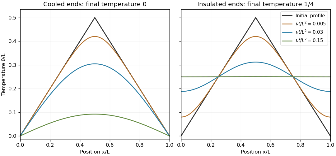
The same triangular initial temperature with cooled and insulated ends
. Original heat-equation solutions for several dimensionless times. Fixed zero-temperature ends cool the bar to zero; insulated ends preserve its initial mean and approach a uniform temperature. Details. Past exam of the mathematics course of the year 2 of the natural sciences course of the University of Cambridge 2004 Paper 1 10 Solution by Codex 0 Created 2026-10-18 Updated 2026-10-20
Codex 0 Created 2026-10-18 Updated 2026-10-20For example, impose homogeneous Dirichlet boundary conditions , and use variations vanishing there. Homogeneous Neumann boundary conditions are another choice removing the boundary terms. Put , , and . At a stationary function let . The quotient rule gives . After integration by parts, stationarity under every allowed variation givesso the fundamental lemma of the calculus of variations yields the stated Sturm-Liouville problem. Conversely an eigenfunction with those boundary conditions has and makes the quotient stationary. The lowest eigenvalue minimizes the Rayleigh quotient under the usual self-adjoint, lower-bounded hypotheses; higher eigenvalues are stationary values with orthogonality constraints when minimizing successively.
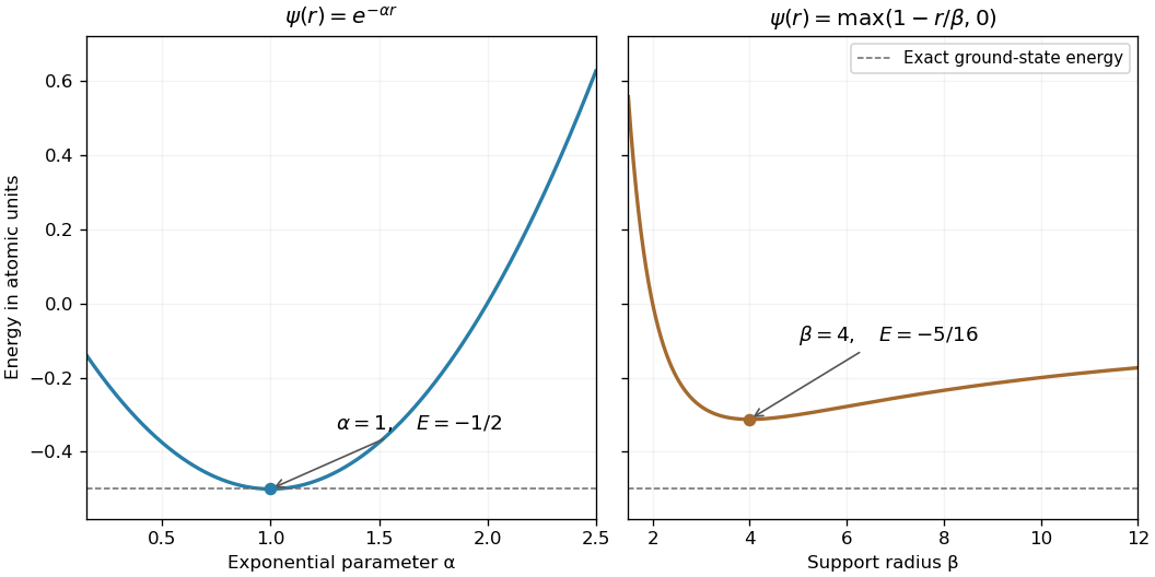
The hydrogen equation becomes . Its radial energy quotient is thereforeRegularity at zero and decay at infinity remove the boundary term . The condition fixes an arbitrary amplitude for these trial functions; it is not their three-dimensional probability normalization, which cancels from the quotient.
For , elementary exponential integrals give , , and . HenceFor the compactly supported linear trial for hydrogen, the norm, gradient and Coulomb integrals are , , and , respectively. ThusThe derivative changes from negative to positive at four, so this is the minimum over positive . The quantum variational principle gives upper bounds on the ground-state energy; the exponential trial is better, and in fact satisfies the exact differential equation at . It is the nodeless hydrogen ground state in the given units. The linear trial is admissible for the energy quadratic form despite its derivative jump at ; it need not possess a classical second derivative at that point.
Past exam of the mathematics course of the year 2 of the natural sciences course of the University of Cambridge 2004 Paper 1 1 Solution by Codex 0 Created 2026-10-18 Updated 2026-10-20
Codex 0 Created 2026-10-18 Updated 2026-10-20Compare the total differential with and . The orthonormality of the coordinate basis gives the gradient in orthogonal coordinates:To obtain the curl without neglecting the variation of the basis vectors, write . The curl of a gradient vanishes, and the product rule givesLikewise because the system is right-handed. This cross product has zero divergence: . The divergence product rule applied to now givesCyclic permutation and linearity give the general component formulas described by divergence and curl from orthogonal coordinate gradients:andIn cylindrical coordinates, . The specified field has no dependence or component, soIt is an irrotational vector field for every exactly when . This statement is local to an angular coordinate chart: the component proportional to is not single-valued under .
Past exam of the mathematics course of the year 2 of the natural sciences course of the University of Cambridge 2003 Paper 2 9 Solution by Codex 0 Created 2026-10-18 Updated 2026-10-20
Codex 0 Created 2026-10-18 Updated 2026-10-20A group homomorphism preserves multiplication: . It sends the identity element to the identity and inverse elements to inverse elements. Its group kernel is . This contains and is closed under multiplication and inverse elements, so it is a subgroup. For and ,Thus ; applying the same argument with gives equality. Hence the group kernel is a normal subgroup.
Let with . The parity of a permutation defines the desired map from :The sign of a permutation is multiplicative, so parity adds modulo two under composition, exactly matching . Thus this is a group homomorphism; it is surjective because a transposition maps to . Its group kernel isThis is the alternating group on three objects, a normal subgroup of index two in .
Past exam of the mathematics course of the year 2 of the natural sciences course of the University of Cambridge 2003 Paper 2 8 Solution by Codex 0 Created 2026-10-18 Updated 2026-10-20
Codex 0 Created 2026-10-18 Updated 2026-10-20A group is a nonempty set with a closed binary operation that is associative, has an identity element, and gives every element an inverse element. A subgroup is a subset that is itself a group under the inherited operation. The left coset of represented by is ; right cosets are defined analogously. Left cosets partition a finite group, and is a bijection from to . Therefore , proving Lagrange's theorem and the required divisibility.
For the given matrices, put and . Since , the generators commute; , , and the generated elements areThey are distinct, and , with exponents reduced modulo four and two. The Cayley table isThe table proves closure and identifies as the identity. The inverse element of is , and associativity follows from matrix multiplication. Thus this is the direct product of cyclic groups of orders four and two, an abelian group of order eight.
Its subgroups are exactlyTo see the list is complete, Lagrange's theorem leaves orders one, two, four and eight. There are exactly three elements of order two, giving the three order-two subgroups. An order-four subgroup containing an element of order four must be one of the two cyclic groups displayed; without such an element it must be the four-element set of elements whose squares are . This is the enumeration in subgroups of C4 times C2.
Past exam of the mathematics course of the year 2 of the natural sciences course of the University of Cambridge 2003 Paper 2 7 i by Codex 0 Created 2026-10-18 Updated 2026-10-20
Codex 0 Created 2026-10-18 Updated 2026-10-20 Past exam of the mathematics course of the year 2 of the natural sciences course of the University of Cambridge 2003 Paper 2 6 b by Codex 0 Created 2026-10-18 Updated 2026-10-20
Codex 0 Created 2026-10-18 Updated 2026-10-20 Past exam of the mathematics course of the year 2 of the natural sciences course of the University of Cambridge 2003 Paper 2 5 Solution by Codex 0 Created 2026-10-18 Updated 2026-10-20
Codex 0 Created 2026-10-18 Updated 2026-10-20The Laplace transform is wherever it converges. For sufficiently large , suitable exponential bounds justify integration by parts and differentiation under the integral sign, givingFor a nonnegative integer and real , substitute in the gamma integral. The result extends holomorphically to , givingThis also follows recursively from the second identity, starting with .
Put , and . For a solution with finite initial values and the required transform bounds, the transformed equation isThe initial-value terms cancel, leaving . On the real interval , a nonzero solution satisfiesIntegration gives . Inverting term by term yieldsTaking gives a nonzero solution, verified by direct substitution. It is , and the rational transform agrees with the general Laplace transform of a Laguerre polynomial. No claim about solutions with singular initial behavior is needed to produce this regular solution.
Past exam of the mathematics course of the year 2 of the natural sciences course of the University of Cambridge 2003 Paper 2 4 Solution by Codex 0 Created 2026-10-18 Updated 2026-10-20
Codex 0 Created 2026-10-18 Updated 2026-10-20Compute the complex derivative along horizontal and vertical increments. Along the real direction, ; along the imaginary direction, . Equality gives the Cauchy-Riemann equationsThe real and imaginary parts of a holomorphic function are smooth. Equality of their mixed partial derivatives then gives and , proving that both are harmonic functions.
For the first real part, and . The Cauchy-Riemann equations require and , so its harmonic conjugate is . ThereforeFor the second real part, is the real part of . Its harmonic conjugate is , givingThese are the most general answers on a connected open domain: the difference of two candidates has zero real part, so the Cauchy-Riemann equations make its imaginary part constant. The second function cannot extend holomorphically through zero.
Past exam of the mathematics course of the year 2 of the natural sciences course of the University of Cambridge 2003 Paper 2 3 Solution by Codex 0 Created 2026-10-18 Updated 2026-10-20
Codex 0 Created 2026-10-18 Updated 2026-10-20Choose the square root of one minus z squared with : explicitly with principal square roots. It is single valued and holomorphic away from the two specified exterior real branch cuts. If for , its boundary values areFor example, above the right cut approaches the negative real axis from below, selecting ; above the left cut approaches it from above, selecting . Continuing once around either branch point changes the sign, which explains the need for cuts.
Apply the residue theorem to on a large disk slit along both cuts, with small arcs excluding . The only enclosed pole is at zero, and its residue is . On the positively oriented boundary of the slit domain, the upper right lip runs from one to , and the lower right lip returns from to one. The jump in gives their combined integral as , where . The left lips similarly give after the substitution .
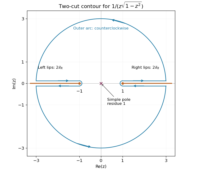
The small arcs contribute because the branch singularities have order . The large arc contributes because . Taking limits therefore yields , and henceThe real substitution independently reduces the integral to , confirming its value and sign.
Past exam of the mathematics course of the year 2 of the natural sciences course of the University of Cambridge 2003 Paper 2 2 Solution by Codex 0 Created 2026-10-18 Updated 2026-10-20
Codex 0 Created 2026-10-18 Updated 2026-10-20Expand the divergence of . The cross terms cancel, leaving . The divergence theorem gives Green's second identity,Use the Green function convention . Integrating over a bounded domain containing yields . Thus zero Neumann boundary data would be incompatible with this unit Dirac delta source. A suitable Neumann Green function with constant boundary flux instead has , where is the boundary area. Substituting , , givesThe last term is an undetermined constant. The data must obey the Neumann Poisson problem compatibility condition , obtained by integrating the original equation. Under this condition an additive constant in cancels from the first two terms.
For the upper half-space, reflect the source to . The method of images with equal-sign sources givesThe reflected singularity lies outside the domain; on the two normal derivatives cancel, so . Its total unit flux passes through a large hemisphere at infinity, where . This is why the bounded-domain condition on the boundary flux cannot be applied to the infinite plane alone.
With zero interior source and the given point boundary source, the boundary representation is . The terms at infinity vanish for this resulting field. ThereforeTo check the singular boundary condition, is the Poisson kernel for the upper half-space. Its integral over a horizontal plane is one and its mass concentrates at the origin as , giving in the distributional sense. This is the Neumann point source on a half-space boundary.
Past exam of the mathematics course of the year 2 of the natural sciences course of the University of Cambridge 2003 Paper 2 1 Solution by Codex 0 Created 2026-10-18 Updated 2026-10-20
Codex 0 Created 2026-10-18 Updated 2026-10-20For a vacuum electric potential, put in Laplace's equation in spherical coordinates. Multiplication by separates the radial and angular terms. With separation constant and , the angular Legendre differential equation isRegularity at both polar axes selects nonnegative integers and the Legendre polynomials. The radial equation is , whose independent solutions are and . Hence the angularly regular axisymmetric vacuum solution isThe radial domain and its boundary conditions determine which terms are admissible.
For the given charge density, only is forced. Write . The interior radial Poisson equation is . The identity for the Poisson equation with a spherical harmonic source gives the particular solution , since the radial operator takes to four. Finiteness at zero and decay at infinity therefore giveContinuity of the electric potential and its radial derivative at requires and . Solving gives , , soAll other angular modes have zero coefficients after imposing regularity, matching and decay. At the origin the interior expression is , which extends with a continuous gradient and value zero. The angular charge density has no unique value exactly at that point; Poisson's equation holds classically for and as a weak solution through the origin. There is no additional point charge.
Pinned article: Introduction to the OurBigBook Project
Welcome to the OurBigBook Project! Our goal is to create the perfect publishing platform for STEM subjects, and get university-level students to write the best free STEM tutorials ever.
Everyone is welcome to create an account and play with the site: ourbigbook.com/go/register. We belive that students themselves can write amazing tutorials, but teachers are welcome too. You can write about anything you want, it doesn't have to be STEM or even educational. Silly test content is very welcome and you won't be penalized in any way. Just keep it legal!
Intro to OurBigBook
. Source. We have two killer features:
- topics: topics group articles by different users with the same title, e.g. here is the topic for the "Fundamental Theorem of Calculus" ourbigbook.com/go/topic/fundamental-theorem-of-calculusArticles of different users are sorted by upvote within each article page. This feature is a bit like:
- a Wikipedia where each user can have their own version of each article
- a Q&A website like Stack Overflow, where multiple people can give their views on a given topic, and the best ones are sorted by upvote. Except you don't need to wait for someone to ask first, and any topic goes, no matter how narrow or broad
This feature makes it possible for readers to find better explanations of any topic created by other writers. And it allows writers to create an explanation in a place that readers might actually find it.
Figure 1. Screenshot of the "Derivative" topic page. View it live at: ourbigbook.com/go/topic/derivativeVideo 2. OurBigBook Web topics demo. Source. - local editing: you can store all your personal knowledge base content locally in a plaintext markup format that can be edited locally and published either:This way you can be sure that even if OurBigBook.com were to go down one day (which we have no plans to do as it is quite cheap to host!), your content will still be perfectly readable as a static site.
- to OurBigBook.com to get awesome multi-user features like topics and likes
- as HTML files to a static website, which you can host yourself for free on many external providers like GitHub Pages, and remain in full control

Figure 2. You can publish local OurBigBook lightweight markup files to either OurBigBook.com or as a static website.
Figure 3. Visual Studio Code extension installation.
Figure 5. . You can also edit articles on the Web editor without installing anything locally. Video 3. Edit locally and publish demo. Source. This shows editing OurBigBook Markup and publishing it using the Visual Studio Code extension. 
- Infinitely deep tables of contents:




All our software is open source and hosted at: github.com/ourbigbook/ourbigbook
Further documentation can be found at: docs.ourbigbook.com
Feel free to reach our to us for any help or suggestions: docs.ourbigbook.com/#contact