By the spectral theorem, the Hermitian matrix $A$ has a complete orthonormal eigenbasis. If $Av=\lambda v$, idempotence gives ${\lambda }^2=\lambda$, so every eigenvalue is zero or one. Since $\det A\ne 1$, at least one is zero. ThereforeThe trace of an idempotent equals its rank; here Hermiticity further identifies $A$ as an orthogonal projection matrix.

A complex inner product $⟨u,v⟩$ is conjugate-linear in its first argument, linear in its second, conjugate symmetric and positive definite: $⟨v,u⟩=\overline{⟨u,v⟩}$ and $⟨u,u⟩>0$ for nonzero $u$. An orthonormal basis is a spanning linearly independent family $e_i$ with $⟨e_i,e_j⟩={\delta }_{ij}$. The associated norm is $\Vert u\Vert =\sqrt{⟨u,u⟩}$.

For two distinct basis elements $x,y$, their orthogonality and unit norms give $\Vert x-y{\Vert }^2=⟨x,x⟩+⟨y,y⟩-⟨x,y⟩-⟨y,x⟩=2$. Hence their distance is $\sqrt{2}$; if the same element is selected twice, it is zero.

Finally, for $B^{†}=B$, the scalar quadratic form obeys $(x^{†}Bx{)}^{\ast }=x^{†}{B}^{†}x=x^{†}Bx$, proving $x^{†}Bx$ is real.

Use the conventionThese are the Fourier transform and inverse Fourier transform for suitably integrable data. Assuming the required ordinary transforms exist and the lower derivatives vanish at both ends, integration by parts gives $\widehat{g^{\prime }}=[g{e}^{-ikx}{]}_{-\infty }^{\infty }+ik\hat{g}=ik\hat{g}$. Repeating this argument yieldsThe decay assumptions are used to discard the boundary terms at each step.

For positive diffusivity $\alpha$, transforming the heat equation gives ${\partial }_t\hat{f}=-\alpha k^2\hat{f}$. Thus $\hat{f}(k,t)=e^{-\alpha k^{2}t}{\hat{f}}_0(k)$, where $f_0(x)=f(x,0)$. The convolution theorem and the Gaussian heat kernel giveFor $f_0(x)=e^{-x^2}$, the Fourier transform of a Gaussian is $\sqrt{\pi }{e}^{-k^2/4}$. Multiplying by the heat factor and inverting gives the Gaussian initial data for the heat equation solutionIt recovers the initial profile as $t\downarrow 0$ and preserves its spatial integral $\sqrt{\pi }$.

Set $T(x,t)=X(x)G(t)$ in the heat equation. Separation of variables gives $G^{\prime }/(c^{2}G)=X^{\prime \prime }/X=-\lambda$. Zero endpoint temperatures impose Dirichlet boundary conditions $X(0)=X(\pi )=0$, selecting $\lambda =n^2$ for $n\ge 1$. The separated factors can therefore be chosen asZero and negative separation eigenvalues give only the zero spatial solution under these boundary conditions.

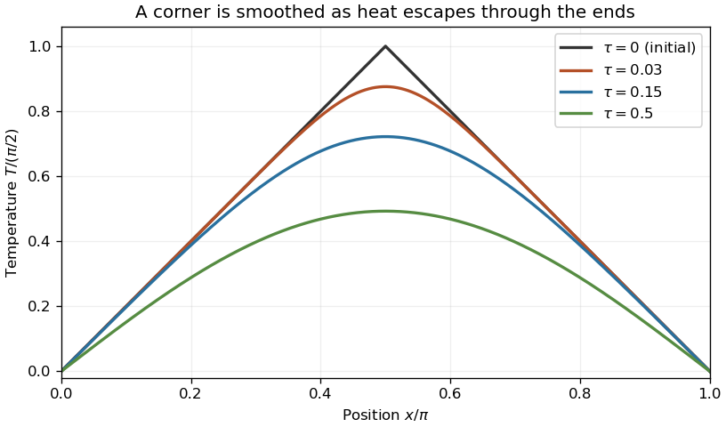
The initial profile is continuous and triangular, with midpoint height $\pi /2$. Its Fourier sine series coefficients areConsequently the heat flow from a triangular initial temperature isFor $t\ge 0$, each summand has magnitude at most $4/[\pi (2m+1{)}^2]$. The Weierstrass M-test proves absolute and uniform convergence. The initial Fourier sine series equals the continuous piecewise smooth profile, and for $t>0$ the exponential factors justify termwise spatial and time differentiation on every time interval bounded away from zero.

Along an extremal, differentiate $f-y^{\prime }{f}_{y^{\prime }}$. The chain rule givesWhen $f_x=0$, the Euler-Lagrange equation makes the right side zero. This proves the Beltrami identity, $f-y^{\prime }{f}_{y^{\prime }}=k$.

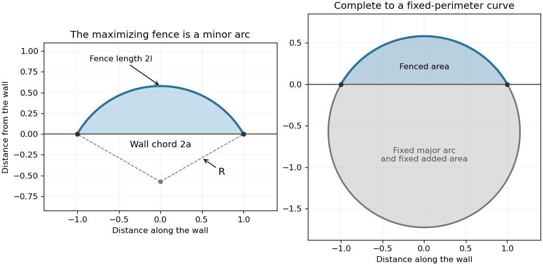
Place the wall on $y=0$ with attachments at $x=\pm a$, and write the fence above it as $y(x)\ge 0$. Maximize area $A={\int }_{-a}^{a}ydx$ subject to length ${\int }_{-a}^a\sqrt{1+y^{\prime 2}}dx=2l$. The isoperimetric constraint gives the augmented integrand $f=y-R\sqrt{1+y^{\prime 2}}$, where $R$ is a constant multiplier. Its Euler-Lagrange equation is $y^{\prime \prime }/(1+y^{\prime 2}{)}^{3/2}=-1/R$, so the fence has constant negative curvature. Equivalently the Beltrami identity is $y-R/\sqrt{1+y^{\prime 2}}=k$.

The resulting maximum-area circular segment with fixed arc length and chord hasHere $0<\theta <\pi /2$ is the half-angle subtended by the arc. Its half-length is $R\theta =l$ and half-chord is $R\sin \theta =a$. The function $\theta /\sin \theta$ increases from one to $\pi /2$, so the given range $a<l<\pi a/2$ determines a unique minor arc. Its enclosed area is $A_{\max }=R^2(\theta -\sin \theta \cos \theta )$.

There is also a global maximality proof for simple fences in the chosen half-plane, without assuming competitors are graphs. Complete the candidate minor arc with the complementary major arc of the same circle, which lies below the wall. Attach this same fixed major arc to any competing fence of length $2l$. The completed closed curve always has perimeter $2\pi R$, and its area is the competitor's fenced area plus the same fixed area below the wall. The planar isoperimetric inequality bounds that total by $\pi R^2$, attained by the candidate circle. Hence no competitor encloses more area, and equality requires the circular arc.

For $r>0$, the chain rule gives $\partial r/\partial x_i=x_i/r$. Differentiating the radial factor gives $d\varphi /dr=e^{ikr}(ikr-1)/(4\pi r^2)$, so in Cartesian coordinatesThe origin is excluded because the scalar field is singular there.

The Stokes theorem states ${\int }_S(\nabla \times \mathbf{F})\cdot \mathbf{n}dS={\oint }_{\partial S}\mathbf{F}\cdot d\mathbf{\ell }$ for a sufficiently smooth vector field and oriented surface with piecewise smooth boundary. The boundary orientation follows the right-hand rule relative to $\mathbf{n}$.

For the convective acceleration identity, use the Levi-Civita symbol contraction ${ϵ}_{ijk}{ϵ}_{k\ell m}={\delta }_{i\ell }{\delta }_{jm}-{\delta }_{im}{\delta }_{j\ell }$. It givesRearranging proves the required vector identity.

For orthogonal coordinates, define the scale factors of orthogonal coordinates $h_i=|\partial \mathbf{r}/\partial q_i|$ and tangent unit vectors ${\mathbf{e}}_i=h_i^{-1}\partial \mathbf{r}/\partial q_i$. They form an orthonormal basis, and $d\mathbf{r}={\sum }_i{h}_i{\mathbf{e}}_{i}d{q}_i$. Equating $d\psi ={\sum }_i{\partial }_{q_i}\psi d{q}_i$ with $\nabla \psi \cdot d\mathbf{r}$ identifies each component. Thus the gradient in orthogonal coordinates isThis holds on a regular coordinate chart where all scale factors are positive.

A right coset of $H$ in $G$ is $Hg=\{hg:h\in H\}$. Right multiplication by $g$ is a bijection $H\to Hg$, with inverse $x\mapsto x{g}^{-1}$, so every right coset has $|H|$ elements. The analogous map $h\mapsto gh$ proves the same assertion for left cosets.

Write the displayed matrices as $M(a,b,c)$. Direct multiplication givesAll new coordinates are integers, so the set is closed. Matrix multiplication is associative, the identity is $M(0,0,0)$, andwhich also has integer coordinates. Thus it is the Integer Heisenberg group.

The subset $H=\{M(0,0,t):t\in \mathbb{Z}\}$ contains the identity, and multiplication and inversion add or negate $t$, so it is a subgroup. Its right cosets areThey are exactly the sets with fixed integer coordinates $(a,b)$, as described by cosets of a coordinate subgroup of the integer Heisenberg group. The factor order $HM$ is essential; multiplying by $H$ on the other side would also change the upper-right coordinate by $at$.

A normal mode has all coordinates following one fixed displacement pattern with a common time factor. Its normal frequency is that factor's oscillation frequency; normal mode coordinates are amplitudes in a basis of such patterns, making the linear equations independent. A zero-frequency mode can instead have constant velocity along a symmetry direction.

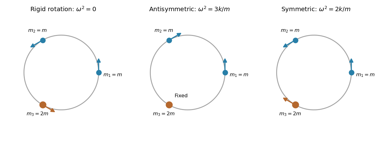
For the unit circle, each angular displacement equals its corresponding arc displacement. The kinetic energy and change in potential energy areAny common spring prestress changes only the constant $V_0$, because the sum of the three arc lengths is fixed. The Euler-Lagrange equations giveThese are the normal modes of three beads connected by springs on a circular hoop, with third mass $M=\mu m$. For $\mu >0$, their three mode vectors and squared angular frequencies areThe zero mode rotates the entire configuration without stretching a spring. The antisymmetric mode moves the equal masses oppositely while leaving the third fixed. In the symmetric mode the equal masses move together against the third, with zero total angular momentum. These vectors are orthogonal in the mass inner product with matrix $m\mathrm{diag}(1,1,\mu )$.

Writing $\mathbf{\theta }=Q_0{v}_0+Q_A{v}_A+Q_S{v}_S$ gives independent equations ${\ddot{Q}}_0=0$, ${\ddot{Q}}_A+{\omega }_A^2{Q}_A=0$, ${\ddot{Q}}_S+{\omega }_S^2{Q}_S=0$. In particular $Q_0=A+Bt$, retaining possible slow common rotation. For $\mu =1$, the two positive frequencies coincide at $\sqrt{3k/m}$; their two-dimensional space is all patterns with ${\theta }_1+{\theta }_2+{\theta }_3=0$.

An isotropic tensor has unchanged components under every rotation of the Cartesian axes. Under proper rotations in three dimensions, rank one has no nonzero isotropic tensor, rank two has $\boxed{T_{ij}=A{\delta }_{ij}}$, and rank three has $\boxed{T_{ijk}=B{ϵ}_{ijk}}$. Here $\delta$ is the Kronecker delta and $ϵ$ the Levi-Civita symbol. If invariance under reflections is also required for a true tensor, the rank-three case vanishes; $ϵ$ is then a pseudotensor.

The velocity gradient tensor for the given field isIts symmetric part, the strain-rate tensor if $\mathbf{u}$ is interpreted as a velocity, isThe antisymmetric part has the specified ordering $D_{ik}-e_{ik}={ϵ}_{ijk}{\omega }_j$, withThe index ordering matters for this sign; it agrees with a local rotation velocity $\mathbf{\omega }\times \mathbf{x}$. This is the axial part of the scalar, symmetric-traceless and axial tensor decomposition, retaining the trace inside the symmetric part here.

At the specified point, $e=\left(\begin{array}{ccc}9& 6& 0\\ 6& 0& 0\\ 0& 0& 4\end{array}\right)$. The upper block has characteristic polynomial ${\lambda }^2-9\lambda -36=(\lambda -12)(\lambda +3)$. Thus the principal values and unit eigenvectors areThese mutually orthogonal directions are the principal strain rates' axes for this local field; reversing an eigenvector does not change its axis.

For causal functions the convolution is $(f\ast g)(t)={\int }_0^{t}f(\tau )g(t-\tau )d\tau$. In a half-plane of absolute convergence, changing variables $u=t-\tau$ in its Laplace transform and using Fubini's theorem givesThis proves the convolution theorem for Laplace transforms. Transforming the differential equation gives $(s^2+1)Y(s)=sy(0)+y^{\prime }(0)+F(s)$. The direct transform pairs $\mathcal{L}(\cos t)=s/(s^2+1)$ and $\mathcal{L}(\sin t)=1/(s^2+1)$ then giveFor a continuous forcing, call the last term $w(t)$. The Leibniz integral rule gives $w^{\prime }={\int }_0^{t}f(\tau )\cos (t-\tau )d\tau$ and $w^{\prime \prime }=f(t)-w(t)$. Also $w(0)=w^{\prime }(0)=0$. Thus both the original equation and the initial values hold.

For an impulse at positive time $T$, the Dirac delta evaluates the convolution, yieldingHere $H$ is the Heaviside step function. The displacement remains continuous at $T$, while its derivative jumps upward by one, exactly as required by integrating the differential equation across the unit impulse.

The residue theorem states that a positively oriented simple closed contour enclosing isolated poles and none on the contour has integral $2\pi i$ times the sum of their residues, provided the function is holomorphic elsewhere inside. Near a simple zero of $\psi$, $\psi (z)={\psi }^{\prime }(a)(z-a)+O((z-a{)}^2)$. HenceFor $\cot z=\cos z/\sin z$, this gives $\boxed{{\mathrm{Res}}_{z=k\pi }\cot z=1}$ for every integer $k$.

To evaluate the real integral, integrate $F(z)=\mathrm{Log}z/(z^2+a^2)$ around an upper semicircle, with a small upper semicircular indentation excluding zero. Use the branch real on the positive axis and with argument between zero and $\pi$ in the upper half-plane. The large arc tends to zero as $O(\ln R/R)$ and the small arc as $O(ϵ|\ln ϵ|)$. The only enclosed pole is $ia$, whose contribution isOn the negative real axis the upper boundary value is $\mathrm{Log}(-x)=\ln x+i\pi$. The two real segments therefore contributeComparing real parts yieldsThe integral is absolutely convergent at both zero and infinity, so no principal-value interpretation is needed.

Use Green's second identity in the source coordinate:Take $u({\mathbf{x}}^{\prime })=\psi ({\mathbf{x}}^{\prime })$ and $v({\mathbf{x}}^{\prime })=-1/[4\pi |\mathbf{x}-{\mathbf{x}}^{\prime }|]$, the fundamental solution of the Laplace equation satisfying ${\Delta }^{\prime }v=\delta ({\mathbf{x}}^{\prime }-\mathbf{x})$. With localized charge and the decaying potential, the boundary integral tends to zero on expanding spheres. The volume identity then gives $\psi (\mathbf{x})+(1/{ϵ}_0)\int vqd{V}^{\prime }=0$, hence the Coulomb potentialConvergence of this integral and a condition fixing the potential at infinity are needed: mere pointwise decay of $q$ is not enough, and a harmonic function could otherwise be added. A bounded, compactly supported charge distribution is a sufficient setting for this derivation.

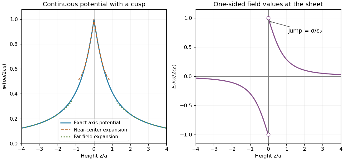
For the disk put $\sigma =Q/(\pi a^2)$. On its axis, every ring of radius $\rho$ is at distance $\sqrt{{\rho }^2+z^2}$, soFor $z>0$ subtract $z$; for $z<0$ add $z$. This is the electrostatic potential of a uniformly charged disk with zero potential at infinity. The absolute value is essential for reflection symmetry and the correct behavior on the lower axis.

For variations $y+ϵ\eta$ with $\eta (a)=\eta (b)=0$, integration by parts gives $\delta I={\int }_a^b[f_y-d(f_{y^{\prime }})/dx]\eta dx$. The fundamental lemma of the calculus of variations therefore gives the Euler-Lagrange equationFor the ramp, use conservation of energy from rest at the rim. The vertical drop is $R\cos \theta$, so $v=\sqrt{2gR\cos \theta }$. The spherical surface arc length is $ds=R\sqrt{d{\theta }^2+{\sin }^2\theta d{\varphi }^2}$. On a monotone segment described by $\varphi (\theta )$, the travel time is consequentlyFor increasing $\theta$ this has the printed limits ${\theta }_0$ to ${\theta }_1$; for a descent, reverse the decreasing angular limits to keep time positive. The azimuth is a cyclic coordinate of this integrand. Its conserved derivative gives the first integral for the brachistochrone on a hemispherical ramp:Solving for its square yieldsFor a regular stationary path with finite $C$, this tends to zero as the rim $\theta \to \pi /2$ is approached. The ratio of azimuthal to meridional displacements is $\sin \theta {\varphi }^{\prime }$, which also tends to zero. Hence the initial direction is along a meridian toward the bottom. This conclusion concerns the initial heading; the later route can turn before reaching the bottom when its rim endpoints require a nonzero azimuthal displacement.