Vary $r$ by $r+\epsilon \eta$ with $\eta (a)=\eta (b)=0$. The first variation of the functional isThe boundary term from integration by parts is zero. The fundamental lemma of the calculus of variations therefore gives $\boxed{F_{1,r}-d{F}_{1,r^{\prime }}/dz=0}$. For $I_2$, independently vary $r$ and $\theta$ with zero endpoint variations; the two Euler-Lagrange equations areFor the optical path, Fermat principle makes $\int \mu ds$ stationary. In cylindrical coordinates its integrand is $L=\mu (r,\theta )s$, with $s=\sqrt{1+r^{\prime 2}+r^2{\theta }^{\prime 2}}$. There is no explicit $z$ dependence. The Beltrami identity for several dependent variables givesThe conserved quantity is the axial component of the optical momentum of a ray. As $\mu >0$, squaring and inverting yieldsNow suppose $\mu =\mu (r)$ and seek a path of radius $R>0$. The angle is a cyclic coordinate, so $L_{{\theta }^{\prime }}=\mu R^2{\theta }^{\prime }/\sqrt{1+R^2{\theta }^{\prime 2}}$ is conserved. At fixed radius this is strictly increasing in ${\theta }^{\prime }$, forcing ${\theta }^{\prime }=\omega$ constant. The radial Euler-Lagrange equation reduces toConsequently the helical rays in a radially graded refractive index haveA real nonzero helix exists at such a radius when $0<-R{\mu }^{\prime }(R)/\mu (R)<1$, and its helical pitch is $2\pi /|\omega |$. If ${\mu }^{\prime }(R)=0$, the solution is instead a straight axial light ray. Thus radial dependence permits constant-radius rays for suitable profiles; an arbitrary radial profile need not support a nonzero real helix. This qualification is necessary, for example when the refractive index increases with radius.

Substitution of $y=x^p$ into the homogeneous Euler-Cauchy equation gives $(p(p-1)+p-1)x^{p-2}=(p^2-1)x^{p-2}$, so $\boxed{p=1,-1}$. Use the solution $u(x)=x$ that vanishes at zero and $v(x)=1/x$ that decays at infinity. Their Wronskian is $u{v}^{\prime }-u^{\prime }v=-2/x$. The half-line Green function for the first cylindrical harmonic is thereforeIt is continuous at $x=s$, its first derivative has jump $1/2-(-1/2)=1$, and it solves the homogeneous equation elsewhere. Thus $L_{x}G=\delta (x-s)$ for integration with ordinary measure $ds$. The boundary conditions hold for each fixed $s>0$.

Integrating against the forcing givesSince the two integrals are $2-(x^2+2x+2)e^{-x}$ and $e^{-x}$, respectively,A Taylor expansion gives $y=-x/2+O(x^2)$ near zero, while $y\sim -1/x$ at infinity. This verifies the two endpoint limits; direct differentiation verifies $Ly=e^{-x}$ on $x>0$. The differential expression itself is singular at zero, so the endpoint condition is imposed by continuity. No nonzero combination of $x$ and $1/x$ satisfies both homogeneous endpoint conditions, proving uniqueness.

Multiplication by $x^2$ puts the eigenvalue problem into Sturm-Liouville form, $-(x^2{y}^{\prime }{)}^{\prime }=\lambda x^{2}y$, with weight $x^2$. If $u,v$ correspond to distinct eigenvalues $\lambda ,\mu$, subtract their multiplied equations and integrate to getThe upper boundary term vanishes by the Dirichlet boundary condition. For a bounded solution near zero, $x^2{y}^{\prime }$ has a limit because $(x^2{y}^{\prime }{)}^{\prime }=-\lambda x^{2}y$ is integrable. A nonzero limit would force a $1/x$ divergence in $y$, so that limit is zero; integration then gives $y^{\prime }=O(x)$. The lower boundary term therefore also vanishes, proving the weighted orthogonality.

Set $z=xy$. For $x>0$, $y^{\prime \prime }+2y^{\prime }/x=z^{\prime \prime }/x$, and finiteness of $y(0)$ gives $z(0)=0$. Thus $z^{\prime \prime }+\lambda z=0$ with zero values at zero and $\pi$. The radial Dirichlet spectrum in three dimensions givesThe zero and negative eigenvalues yield only the zero solution under these boundary conditions. Also ${\int }_0^{\pi }{x}^2{y}_n^{2}dx=\pi /2$.

For the forced equation, the same substitution gives $z^{\prime \prime }-\beta z=x$. The Fourier sine series of $x$ on $(0,\pi )$ has coefficientsExpanding $z=\sum c_n\sin nx$ gives $-(n^2+\beta )c_n=b_n$, henceThe value at zero is defined by a limit. In fact $|\sin nx/x|\le n$, so uniform convergence holds even there, by comparison with $2\sum (n^2+\beta {)}^{-1}$. An independent check comes from solving the constant-coefficient equation directly:It satisfies both endpoint conditions and the forcing for $x>0$, and its finite origin limit agrees with the series. For $\beta >0$ the homogeneous boundary value problem has no nonzero solution, so the solution is unique.

For the normalized second-order linear differential equation $y^{\prime \prime }+P(z)y^{\prime }+Q(z)y=0$, an ordinary point $z_0$ has analytic $P,Q$ near $z_0$. At a regular singular point, which is not ordinary, $(z-z_0)P(z)$ and $(z-z_0{)}^{2}Q(z)$ are analytic. Ordinary points admit two independent convergent power series solutions. Regular singular points instead call for the Frobenius method, which permits leading powers and, in some cases, logarithms.

Here zero is an ordinary point. Substitute $y={\sum }_{n\ge 0}{a}_n{z}^n$ into the Hermite differential equation and equate coefficients:The even and odd initial coefficients are independent, givingThese are the power series solutions of the Hermite differential equation, with the present parameter equal to twice the parameter in that article. The ratio of successive terms within each nonterminating parity is asymptotically $2|z{|}^2/n$, so both series have infinite radius of convergence.

For a nonzero polynomial of degree $m$, its highest coefficient in $-2z{y}^{\prime }+\lambda y$ forces $\lambda =2m$. Conversely at that value the matching parity terminates. HenceThe polynomial solutions are scalar multiples of the Hermite polynomials. Two examples are $\boxed{\lambda =0:y=1;\lambda =2:y=z}$; direct substitution verifies both. The other independent solution generally remains nonpolynomial.

The spectral theorem gives a real orthonormal eigenbasis $v_1,\dots ,v_n$ for a real symmetric matrix $A$. Distinct eigenspaces are orthogonal; within a repeated eigenspace, choose an orthonormal basis, for example by Gram-Schmidt orthogonalization. Put these eigenvectors in the columns of $T$. Then $T^{-1}=T^T$ andFor a change of variables $y=Sx$, choose $\boxed{S=T^T}$. Since $x=Ty$, the quadratic form becomes $x^{T}Ax={\sum }_i{\lambda }_i{y}_i^2$; the ${\lambda }_i$ are precisely the eigenvalues of $A$.

In the numerical case, the off-diagonal entries are half the cross-term coefficients, soA direct eigenvector calculation gives the unit eigenvectors $(1,1,0)/\sqrt{2}$, $(1,-1,1)/\sqrt{3}$, $(1,-1,-2)/\sqrt{6}$, with eigenvalues two, three and minus six. They are pairwise orthogonal. Therefore the required orthogonal diagonalization isand the transformed quadratic form is $\boxed{2y_1^2+3y_2^2-6y_3^2}$.

Use the Fourier transform convention $\hat{f}(k)={\int }_{\mathbb{R}}f(t)e^{-ikt}dt$, with inverse factor $1/(2\pi )$. For functions in L1 space, their convolution is $h(t)={\int }_{\mathbb{R}}f(s)g(t-s)ds$. Fubini's theorem applies because the absolute double integral is $\Vert f{\Vert }_1\Vert g{\Vert }_1$. Substituting $r=t-s$ therefore proves the convolution theorem:For the specified rectangular pulse, the support condition is $|t|<1$. Its Fourier transform isThe convolution $f\ast f$ is the length of the overlap of $(-1,1)$ and $(t-1,t+1)$. Thus it is the triangular pulseThe transform's value at zero is four, given by its continuous extension. In this convention, the Parseval identity for square-integrable functions isFor the rectangular pulse the left side is two, giving the sinc-squared integralFor the triangular pulse, $\int |f\ast f{|}^{2}dt=2{\int }_0^2(2-t{)}^{2}dt=16/3$. Apply the same Parseval identity with transform $4{\sin }^{2}k/k^2$ to obtain the sinc fourth-power integralBoth integrands have removable singularities at zero and integrable tails.

Choose homogeneous Dirichlet boundary conditions, $y(a)=y(b)=0$, and nonzero admissible functions with finite $F$ and positive $G$. Variations obey the same zero endpoint values. At a stationary Rayleigh quotient, set $\lambda =F[y]/G[y]$. ThenThe boundary term vanishes, and the fundamental lemma of the calculus of variations gives the Sturm-Liouville equation $-(p{y}^{\prime }{)}^{\prime }+qy=\lambda wy$. Thus stationary functions are eigenfunctions. Conversely, multiply that equation by $y$ and integrate by parts to obtain $F=\lambda G$; its first variation then vanishes by the same calculation. This proves that stationary values are the corresponding eigenvalues. Homogeneous Neumann boundary conditions also make the displayed boundary terms vanish; general Robin boundary conditions can require a boundary contribution to the quadratic form.

For $p=1$, $q=0$, $w=x$ on $(0,\pi )$, the polynomial trial function $y=x(\pi -x)$ satisfies the endpoint conditions. Its Rayleigh quotient usesso the polynomial estimate is $\boxed{{\lambda }_{\mathrm{poly}}=20/{\pi }^3\simeq 0.64503}$. The trigonometric trial function $y=\sin x$ givesand hence $\boxed{{\lambda }_{\mathrm{trig}}=2/\pi \simeq 0.63662}$. Both are upper bounds on the lowest eigenvalue, by the Rayleigh-Ritz method; neither trial is an exact eigenfunction, so the inequalities are strict.

Their closeness has a useful explanation beyond their similar single-arch shapes. Both trial functions are symmetric under $x\mapsto \pi -x$, forcing ${\int }_0^{\pi }x{y}^{2}dx=(\pi /2){\int }_0^{\pi }{y}^{2}dx$. The reflection-symmetric trials for a linearly weighted Rayleigh quotient therefore reduce this problem to a constant multiple of the ordinary Dirichlet energy quotient. The sine is the best trial within this symmetric class, and the polynomial's value is only a factor $10/{\pi }^2\simeq 1.0132$ larger. The unrestricted lowest eigenfunction can be asymmetric because the weight $x$ is asymmetric.

For $a>0$, the positive constant-$u$ surfaces in elliptic cylindrical coordinates satisfyThey are confocal elliptic cylinders with focal lines $x=\pm a,y=0$. For a generic fixed $v$, eliminating $u$ givesBecause $u\ge 0$, a fixed $v$ selects the half-branch with the signs of $x$ and $y$ fixed by $\cos v$ and $\sin v$. These are hyperbolic cylinders. The degenerate $u=0$ surface is $y=0$, $|x|\le a$, extended in $z$. At $v=0,\pi$ the cross-sections are the two exterior horizontal rays; at $v=\pi /2,3\pi /2$ they are vertical half-axes.

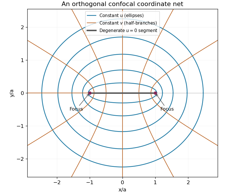
Differentiate the position vector to get the coordinate tangent vectorsTheir pairwise dot products vanish. Their squared lengths are $a^2({\sinh }^{2}u+{\sin }^{2}v)$, $a^2({\sinh }^{2}u+{\sin }^{2}v)$ and one. This proves orthogonality and gives the scale factors of orthogonal coordinates:The Riemannian metric is $d{s}^2=h^2(d{u}^2+d{v}^2)+d{z}^2$. Away from the focal lines, divide the coordinate tangent vectors by their lengths to obtain the local orthonormal unit vectors $e_u,e_v,e_z$. For physical vector field components $A_u,A_v,A_z$, the formulas for vector calculus in elliptic cylindrical coordinates areThe gradient of a scalar function has components $({\varphi }_u/h,{\varphi }_v/h,{\varphi }_z)$. Apply the divergence formula to this gradient; Laplace's equation becomesThe formulas apply where $h>0$; the focal lines require a limit or another coordinate chart.

Conjugacy classes. For $a\in G$, its conjugacy class isEvery element belongs to its own conjugacy class, by taking $g=e$. To prove uniqueness, suppose $x=ga{g}^{-1}=hb{h}^{-1}$ belongs to both $\mathrm{Cl}(a)$ and $\mathrm{Cl}(b)$. ThenFor every $t\in G$, this makes $tb{t}^{-1}$ a conjugate of $a$ as well. Hence $\mathrm{Cl}(b)\subseteq \mathrm{Cl}(a)$, and reversing the argument gives the other inclusion. Two conjugacy classes that meet are therefore equal, proving that the classes partition $G$.

Abelian case. If $G$ is an abelian group, then $ga{g}^{-1}=ag{g}^{-1}=a$ for every $g$, so $\boxed{\mathrm{Cl}(a)=\{a\}}$ for each $a$.

Centre. An element has a singleton conjugacy class precisely when $gz{g}^{-1}=z$ for every $g$, equivalently $gz=zg$ for every $g$. Thus the definition in the paper agrees with the usual centre of a group:The identity lies in $Z(G)$. If $z,w\in Z(G)$, then for any $g$, $gzw=zgw=zwg$, so $zw\in Z(G)$. Also $gz=zg$ implies $z^{-1}g=g{z}^{-1}$, so $z^{-1}\in Z(G)$. This proves it is a subgroup. Any two of its elements commute because either one commutes with every element of $G$. Consequently $\boxed{Z(G)\text{ is an abelian subgroup of }G}$.

Square symmetry. Use the paper's notation $D_4$ for the eight-element dihedral group of a square. Let $r$ be a quarter-turn and $s$ a reflection, so $r^4=s^2=e$ and $srs=r^{-1}$. A rotation $r^j$ commutes with $s$ exactly when $r^j=r^{-j}$, or $2j=0$ modulo four. This selects $e$ and $r^2$. No reflection $r^{j}s$ commutes with $r$, becauseand $r^{j-1}\ne r^{j+1}$. Therefore

Cosets and counting. A left coset of a subgroup $H$ in a group $G$ is $gH=\{gh:h\in H\}$. The left cosets partition $G$ and each has $|H|$ elements. Lagrange's theorem states that for a finite group, $\boxed{|G|=[G:H]|H|}$; in particular, the subgroup order divides the group order.

The matrix group. Work throughout in the finite field ${\mathbb{F}}_5$, so every nonzero entry has a multiplicative inverse. Denote a matrix by $A(a,b,c)$, with $a,c\ne 0$. Ordinary matrix multiplication, interpreted using modular arithmetic, givesIts diagonal entries remain nonzero, proving closure. Associativity is inherited from matrix multiplication, $A(1,0,1)$ is the identity element, andThis lies in the same set and multiplication checks the inverse in either order. Thus these matrices form a group. There are four choices each for $a$ and $c$ and five for $b$, giving $\boxed{|G|=4\cdot 5\cdot 4=80}$.

The subgroup. Write $h(a,c)=A(a,a-c,c)$. ThenIt contains the identity $h(1,1)$, is closed, and has inverse $h(a^{-1},c^{-1})$. Interchanging the two factors leaves the product unchanged because multiplication in ${\mathbb{F}}_5$ is commutative. Therefore $H$ is an abelian subgroup, withEquivalently $H$ is isomorphic to ${\mathbb{F}}_5^{\times }\times {\mathbb{F}}_5^{\times }$ by $h(a,c)\mapsto (a,c)$, which also explains its abelian property. Its order divides $80$, verifying Lagrange's theorem.

There are five distinct left cosets. Representatives can be taken as $U_t=A(1,t,1)$, $t\in {\mathbb{F}}_5$: indeedEvery matrix lies in exactly the coset specified by this unique $t$.

Elements whose square is the identity. Squaring givesThus $a,c\in \{1,-1\}=\{1,4\}$ and $b(a+c)=0$. For equal signs, $a+c\ne 0$ in ${\mathbb{F}}_5$, so $b=0$. For opposite signs, $a+c=0$ and all five $b$ values work. The complete set is thereforeIt contains $2+5+5=12$ elements, including the identity; the other eleven are involutions. Since $12$ does not divide $80$, Lagrange's theorem proves that this set is not a subgroup.