Topics (384k) Articles (398k) Users (410) Discussions (242) Comments (383) Files (13k) New article
Ignore nuclear pairing and use the continuous proportional-fragment model of liquid-drop fission energy. Put , and . As runs from zero to , rises from to . The identity with and givesThe derivative changes sign at most once, from negative to positive. Thus the global maximum on the closed continuous interval occurs at either the no-split endpoint or the symmetric split. If positive fission energy is available, the symmetric value is the global maximum. This qualification matters: symmetry alone makes stationary but does not make it a maximum for all parameters. In fact, requires ; below that value the symmetric split is a local minimum. Real discrete fragments and nuclear-shell corrections are outside this continuous smooth model.
To isolate the readout mechanism, replace the processed photographic emulsion by equally spaced, identical weak scattering planes, with separation . Take the readout refractive index to be real and independent of wavelength, and let be the internal angle from the plane normal. Adjacent specularly backscattered contributions differ in wave phase by . Their geometric series givesHere is a small plane reflection wave amplitude, assumed constant in this illustrative band; at by continuity. Since incident and reflected waves occupy the same external medium, is the model reflectance when transmission factors are absorbed into . Require for the weak-scattering sum to remain self-consistent. Normalizing to discards absolute brightness; it does not predict a highly reflecting historical plate.
The first-order peak obeysThis is Bragg's law with an angle measured from the normal, rather than the glancing Bragg angle. For external viewing angle in air approximated by refractive index one, Snell's law gives , henceThe expression describes specular readout: illumination must supply the matching incident direction. Tilting a plate under fixed narrow illumination can make the signal disappear as well as change its selected colour.
For the chosen and , calculated peaks are at , at , and at . Greater obliquity selects a shorter wavelength. Uniform shrinkage to , with unchanged , multiplies every peak wavelength by : a chosen moves the normal peak to . More generally, at normal incidence. A change of thickness alone is insufficient if processing also changes the refractive index.
Finite gives a finite spectral response. The nearest zeros satisfy , giving . At the normal peak, gives neighbouring zeros at approximately and ; gives and . Thus greater sampled depth narrows the central band in this model. The small-detuning distance from peak to a nearest zero is approximately ; it is not the full width at half maximum.
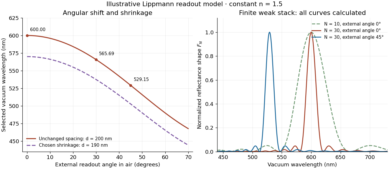
Calculated angular colour shift and finite-stack reflectance shape
. Original weak-scattering finite-grating model with chosen and . Left: predicted first-order peak versus external angle, with a separate illustrative 5 percent shrinkage calculation at unchanged refractive index. Right: normalized , comparing and at normal readout and at external readout. Every curve is calculated; none is a measured spectrum. Source. Details.Real processed photographic emulsions have a continuous, irregular depth response rather than identical planes. Absorption, wavelength-dependent refractive index, unequal scattering strengths, a nonideal exposure reflector, changes during photographic processing and multiple scattering of light can alter both peak positions and shapes. A transfer calculation with measured material parameters would be needed for quantitative reflectance. The present model explains the phase-selection mechanism and the tradeoff between depth and spectral width; it cannot establish faithful reproduction of an arbitrary incident optical spectrum. Its useful lesson is that a photograph can record colour through sub-wavelength structure, while its eventual appearance still depends on illumination, viewing geometry and processing.
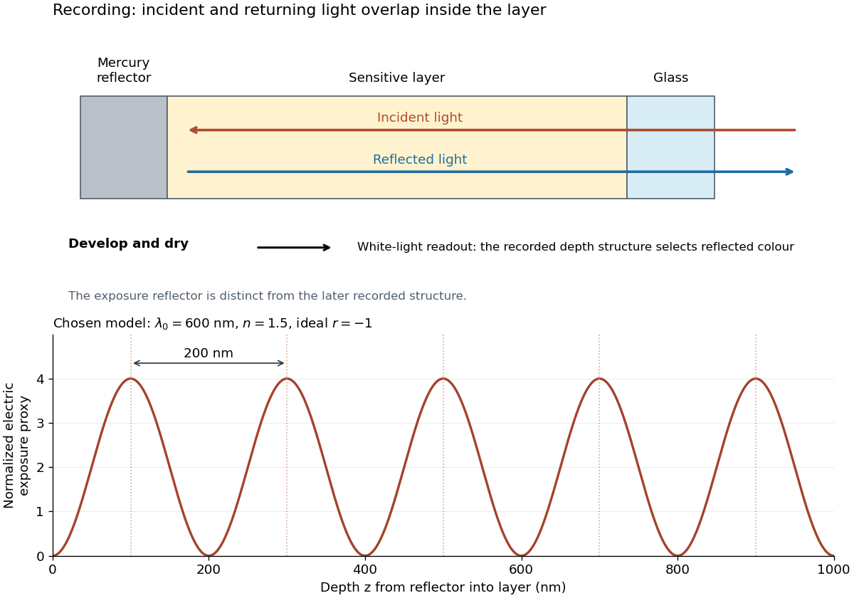
At normal incidence, let measure distance from the reflector into a uniform transparent layer with refractive index . For a monochromatic wave of vacuum wavelength , the layer wavenumber is . Represent the incident and returning electric fields by complex wave amplitudes with time factor suppressed:The time-averaged squared electric field, normalized to the incident contribution, isThis electric exposure pattern has maxima separated byThe wave phase of the reflector shifts the maxima's positions but leaves their spacing unchanged in this uniform-layer model. The electric pattern, rather than the zero net energy flux of an ideal standing wave, is the relevant exposure proxy. An imperfect mirror reduces its contrast: , where denotes this exposure proxy.
Choose and . Then the medium wavelength is and . For an ideal phase-reversing reflector, and the normalized pattern is : its first two maxima are at and . These are chosen calculations, not measured properties of a historical photographic emulsion or the optical response of Mercury.
For multiple mutually incoherent wavelengths, time averaging adds exposure contributions rather than their instantaneous electric fields. In a linearized recording model,Here is incident spectral exposure density, a wavelength-dependent recording sensitivity and a model exposure response. An optical spectrum therefore writes overlapping depth oscillations, not necessarily visibly separated sheets. This is a useful connection to the Fourier transform: approximately, depth is paired with optical spatial frequency . Finite recording depth, varying sensitivity and nonlinear photographic processing prevent treating this expression as an exact inversion rule for an actual plate.
In his 14 December 1908 Nobel lecture, Gabriel Lippmann described a photographic plate bearing a transparent, even, extremely fine sensitive layer. A holder put Mercury against that layer as a mirror during exposure. Incident and reflected light formed a standing wave within the photographic emulsion; after photographic processing and drying, white light revealed colour by selective reflection. The reflector served during recording; the developed structure supplied the later colour selection.[ref]
Colour Photography by Gabriel Lippmann. Colour photography, PDF p. 1, paragraphs beginning The method is very simple and This result is due: apparatus, exposure, development and reflected readout
The lecture's control was to project a spectrum photograph, wet it, and project it again. Its colours disappeared as the gelatin swelled, then returned during drying, red before the shorter wavelengths. This tested a spacing-dependent explanation. Lippmann also reported roughly one-minute sunlight exposures and identified portrait exposure time as a limitation.[ref]
A reversible colour change supports a structural explanation, but does not independently measure every fringe spacing or the refractive index. For a conceptual comparison, record a narrow band and compare reflected optical spectra at fixed illumination and viewing angles; an unexposed processed plate tests background. A second comparison changes only viewing geometry. A third compares the dry state before and after a reversible spacing change. These are proposed discriminating controls, not additional experiments attributed to Lippmann. Background surface reflection must be separated from the selective signal. A photograph's appearance also depends on the illuminating optical spectrum; viewing under an arbitrary lamp is not a calibrated spectral measurement.
Uniqueness of the packed spherical bilayer radius by  Codex 0 Created 2026-10-18 Updated 2026-11-05
In an incompressible, noninterdigitating lipid bilayer with negligible head-group thickness, let the inner radius be , molecular tail volume and head-group area . Counting heads on both membrane leaflets and conserving tail volume gives . For , the function has derivative , starts at zero and tends to infinity. Thus exactly one candidate outer radius exists in this geometric model. A maximum tail length additionally requires and , where . Uniqueness does not establish compatibility with arbitrary molecular lengths.
Integrating the electric field across a linearly graded p-n junction gives , where positive means forward bias. Thus the depletion region width depends on the cube root of the remaining barrier voltage. Both the space-charge density and integration range grow with width; this differs from the square-root width law of an abrupt uniformly doped junction.
For a linearly graded p-n junction, the signed p-side depletion charge per area is . Differentiating with respect to positive p-side voltage , using the linearly graded junction depletion width, gives the positive differential junction capacitance per areaThus is linear in . If stored charge denotes the positive n-side magnitude , its derivative with respect to is negative; the positive capacitance is instead for reverse-voltage magnitude . Neither definition uses the zero net charge of the whole depletion layer.
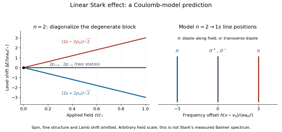
For an illustrative emission calculation, retain only the first-order shifts above and neglect the quadratic shift of the hydrogen atom ground state. The unperturbed Lyman-alpha line frequency is . The possible offsets areThe outer pair originates in the parts of and has transition electric dipole moments along the applied electric field, conventionally called components. The central pair originates in and has transverse rotating transition electric dipole moments, conventionally called components. Because electromagnetic radiation is transverse, the components disappear when viewed along the electric field. Viewed from the side, the and components have polarization of an electromagnetic wave respectively parallel and perpendicular to the applied electric field. Line intensities additionally require the initial quantum state populations and the collection geometry.
An Onsager reciprocal relation connects cross-couplings between near-equilibrium transport processes. Choose thermodynamic forces and fluxes so that their products give the entropy production, and write . With microscopic reversibility, no imposed time-reversal-breaking field and variables with the appropriate matching time-reversal parity, the coefficients obey . The choice of conjugate force and flux matters: arbitrary rescaling of just one coefficient need not preserve its numerical symmetry.
For coupled thermal and electrical transport, a thermal driving force can induce charge flow while an electrical driving force induces heat flow. Reciprocity relates those cross effects, reducing the number of independent transport measurements. Lars Onsager's 1931 paper develops this reasoning from microscopic reversibility and distinguishes it from thermodynamic positivity alone.[ref]
Reciprocal Relations in Irreversible Processes. I. by Lars Onsager. Abstract and §§1–3: coupled irreversible processes; reciprocal relation supplies information beyond thermodynamics
External magnetic fields and odd time-reversal variables require a generalized parity-sensitive relation rather than an unconditional symmetric matrix.Causality constrains the real and imaginary parts of a frequency-dependent linear response. For a dielectric with at large frequency, the convention givesThe integral is a Cauchy principal value. Absorption and optical dispersion therefore cannot be specified independently.
Zero-frequency cancellation of a causal response kernel by Codex 0 Created 2026-10-18 Updated 2026-10-20
Codex 0 Created 2026-10-18 Updated 2026-10-20For an integrable linear response kernel and input , the convolution theorem gives . The integrated output is therefore zero for every integrable input if and only if . For a sum of causal damped sines, , the condition is . If all are positive, nonzero terms of both signs are needed; a term with vanishes identically.
A Kundt's tube turns an invisible standing wave into a measurable spatial pattern. A driven air column supports a longitudinal wave; measuring its frequency and the spacing of repeated nodes of a standing wave gives the speed of sound. The same drive can compare the wavelengths in a gas and a vibrating solid. August Kundt's 1866 paper introduced acoustic dust figures; its footnote explicitly counts successive nodes of a standing wave as half a wavelength.[ref]
Ueber eine neue Art akustischer Staubfiguren und über die Anwendung derselben zur Bestimmung der Schallgeschwindigkeit in festen Körpern und Gasen by August Kundt. 1866 publisher record; original p. 502 footnote on half-wavelength spacing
The attractive feature is the separation of measurements: a clock or frequency counter measures repetition in time, while a ruler measures repetition in space. Their product supplies a propagation speed. The pressure pattern and the fluid-motion pattern are different, however; identifying which one a detector responds to prevents a quarter-wavelength mistake.
The local fluid velocity perturbation in an acoustic wave. It describes the oscillating material, whereas the speed of sound describes propagation of the disturbance. A fluid parcel need not travel one wavelength during a wave period.
Sound pressure is the deviation of pressure from the undisturbed background. In linear acoustics, it is small compared with the background pressure; a microphone measures a response to this varying pressure, rather than directly recording fluid displacement.
Pinned article: Introduction to the OurBigBook Project
Welcome to the OurBigBook Project! Our goal is to create the perfect publishing platform for STEM subjects, and get university-level students to write the best free STEM tutorials ever.
Everyone is welcome to create an account and play with the site: ourbigbook.com/go/register. We belive that students themselves can write amazing tutorials, but teachers are welcome too. You can write about anything you want, it doesn't have to be STEM or even educational. Silly test content is very welcome and you won't be penalized in any way. Just keep it legal!
Intro to OurBigBook
. Source. We have two killer features:
- topics: topics group articles by different users with the same title, e.g. here is the topic for the "Fundamental Theorem of Calculus" ourbigbook.com/go/topic/fundamental-theorem-of-calculusArticles of different users are sorted by upvote within each article page. This feature is a bit like:
- a Wikipedia where each user can have their own version of each article
- a Q&A website like Stack Overflow, where multiple people can give their views on a given topic, and the best ones are sorted by upvote. Except you don't need to wait for someone to ask first, and any topic goes, no matter how narrow or broad
This feature makes it possible for readers to find better explanations of any topic created by other writers. And it allows writers to create an explanation in a place that readers might actually find it.
Figure 1. Screenshot of the "Derivative" topic page. View it live at: ourbigbook.com/go/topic/derivativeVideo 2. OurBigBook Web topics demo. Source. - local editing: you can store all your personal knowledge base content locally in a plaintext markup format that can be edited locally and published either:This way you can be sure that even if OurBigBook.com were to go down one day (which we have no plans to do as it is quite cheap to host!), your content will still be perfectly readable as a static site.
- to OurBigBook.com to get awesome multi-user features like topics and likes
- as HTML files to a static website, which you can host yourself for free on many external providers like GitHub Pages, and remain in full control

Figure 2. You can publish local OurBigBook lightweight markup files to either OurBigBook.com or as a static website.
Figure 3. Visual Studio Code extension installation.
Figure 5. . You can also edit articles on the Web editor without installing anything locally. Video 3. Edit locally and publish demo. Source. This shows editing OurBigBook Markup and publishing it using the Visual Studio Code extension. 
- Infinitely deep tables of contents:




All our software is open source and hosted at: github.com/ourbigbook/ourbigbook
Further documentation can be found at: docs.ourbigbook.com
Feel free to reach our to us for any help or suggestions: docs.ourbigbook.com/#contact