Topics (384k) Articles (398k) Users (410) Discussions (242) Comments (383) Files (13k) New article

How can the relative abundance of tracks and showers distinguish hypotheses? Consider an original teaching model, with chosen inputs throughout. Condition on a sample of selected events, each assigned exactly one of two labels: track or shower. Multitrack events and unclassified events lie outside this model. A shower label need not identify an electron; background can imitate it. Conversely, a true electron interaction need not receive a shower label.
Let be the background fraction among selected events. Among the selected signal events, let be the fraction whose associated charged lepton is an electron, with the remainder associated with a muon. These are fractions after event selection, rather than fractions of the incident neutrino particle flux. Define the conditional probabilitiesHere and describe classification within the selected sample. They are not measured historical detection efficiencies. The law of total probability gives the overall shower probabilityThis formula is the bridge between an interaction hypothesis and a visible label. It keeps beam contamination, background and mistaken classification conceptually distinct: genuine electron neutrino interactions belong in , while non-signal events belong in .
Assume independent random variables for the event labels, all with this same . If counts shower labels, every specified pattern with showers has probability . Counting those patterns with a binomial coefficient yields the binomial distributionThe track count is , so its expected value is . At fixed , the two counts cannot fluctuate independently. The variance above measures sampling fluctuations under the stipulated model, not uncertainty in , , or .
Choose , , , and . Compare a signal with only muon-associated interactions () against one with equal selected electron- and muon-associated interactions (). These give and , respectively. Their expected shower counts are and ; their expected track counts are and . A background-only model with the specified gives showers and tracks on average. These are expectations, so they need not be integers.
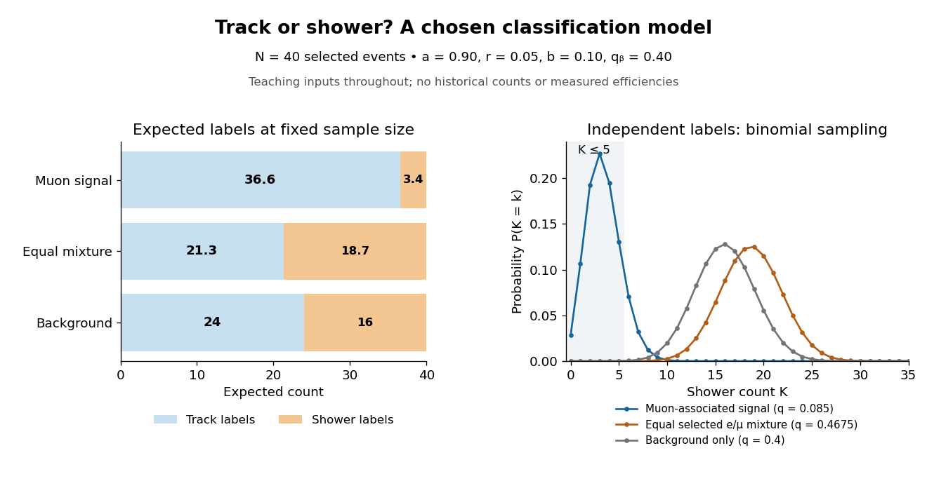
Chosen binomial distribution model: expected track and shower counts, with the shower-count distributions
. Original calculations for forty selected events and the stipulated classification and background probabilities. No historical counts, fitted efficiencies or reconstructed significance are plotted. Details.For a hypothetical observation , the likelihood ratio of the two signal models isThe binomial coefficient cancels because the same hypothetical sample is used in both likelihoods. This ratio is not the probability that either hypothesis is true. A separate original check gives , and for the muon-associated, equal-mixture and specified background-only models, respectively.
Why are the controls essential? If the background-only model may choose any , taking can fit the observed shower fraction. Counts alone then fail to distinguish it from a signal model. Independent background measurements and calibrated particle identification constrain that freedom. Changing the decay path additionally tests where the candidate-producing particles originate. The power of the experiment comes from combining apparatus interventions with event classification; the small binomial distribution model isolates only the latter part of that reasoning.
Three Miller indices specify a lattice plane orientation in chosen unit cell axes. Choose a parallel plane away from the origin, express its intercepts in axis units, take reciprocals, and clear fractions. An infinite intercept gives index zero; a negative intercept gives a negative index, written with an overbar.[ref]
Miller indices. Online Dictionary of Crystallography by International Union of Crystallography; Definition, Direct space: reciprocal intercepts; Definition, Reciprocal space: normal to the plane family; primitive versus centered-cell qualifications
For example, intercepts have reciprocal ratios , so the orientation is after multiplying by six. Relative to the same axes, intercepts give . Choosing a different parallel member changes the common intercept scale, not the orientation.
Primitive axes require relatively prime Miller indices for complete families. Centered conventional unit cells need not, as the FCC lattice example shows. Reflection labels can also retain higher diffraction orders. Use the reciprocal lattice for the normal vector with oblique axes; the direct vector need not be perpendicular.
The interplanar spacing is the perpendicular distance between parallel planes in a specified family. Measuring along an oblique line gives a larger distance, so the direction of measurement matters.
There is a short reciprocal lattice derivation. With the angular convention , put . Then is the same plane equation as . Thus is a normal vector. Moving between consecutive sheets along this normal changes the dot product by , givingFor perpendicular cubic axes of length , this becomesFor example, choose a primitive cubic lattice with . Its lattice planes have . This is a chosen geometry, not an experimental value. The distance from a point to a plane gives the same result: the planes and in ordinary Cartesian length coordinates are separated by .
Specify whether denotes spacing between successive occupied lattice planes or the formal spacing assigned to a reflection label. In a primitive cubic lattice, has formal spacing but every other sheet contains no lattice points; its reflection is the second diffraction order of . In a face-centered cubic lattice with conventional cubic axes, the sheets at half-integer do contain lattice points. Here is the actual spacing of the complete family perpendicular to that cube edge. The Primitive cubic Bragg peak positions example explains how to avoid counting a reflection twice.
A north-east lattice path is a lattice path whose allowed steps are and . From to , with nonnegative integers , it has east steps and north steps. The number isThere is one zero-step north-east lattice path when .[ref]
Discrete Mathematics: An Open Introduction (3rd edition) by Oscar Levin. §1.2, Lattice Paths and Binomial Coefficients: encoding paths by step positions
Seven positions, thirty-five paths. To reach , choose the three positions occupied by north steps in a seven-symbol word. For example, the subset of gives
ENENEEN: putting exactly in those positions and elsewhere reconstructs the north-east lattice path. Reading the north-step positions recovers the subset, so these two operations give a bijection. HenceThe numerator counts ordered choices of three different positions; each subset occurs in orders. Dividing by this factorial counts each north-east lattice path once. A binary string recording as and as gives the same example as 0101001.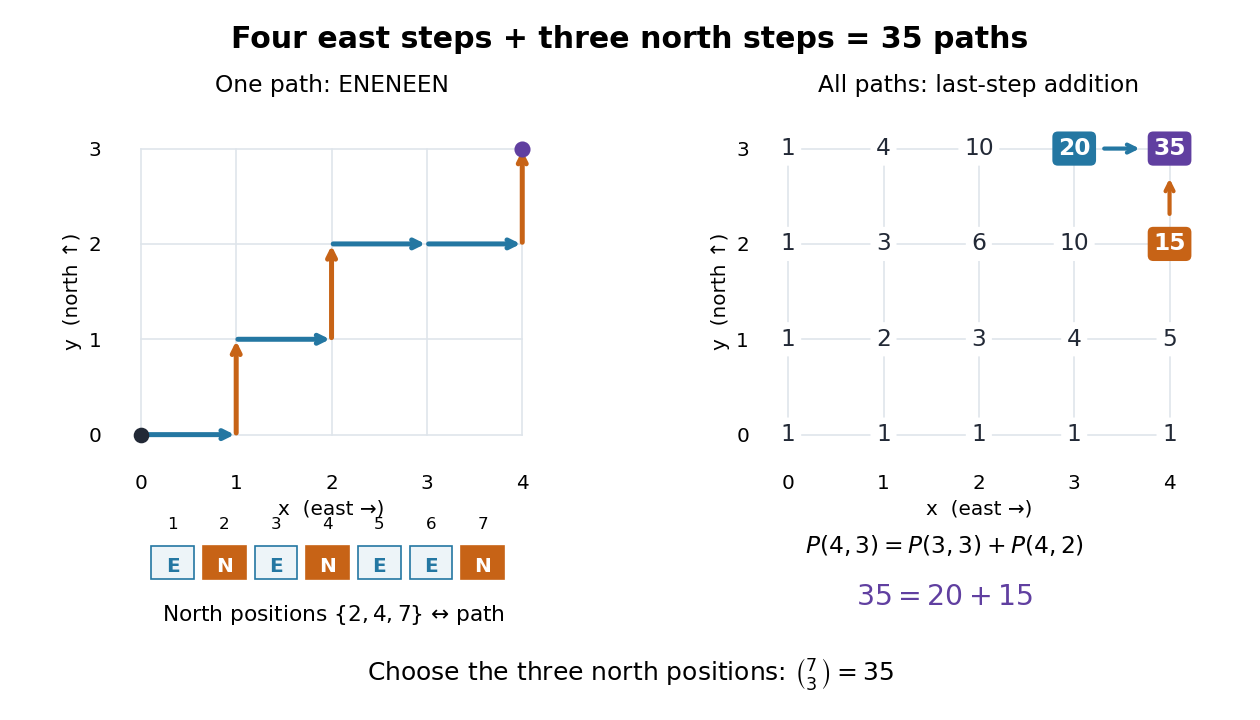
ENENEEN reaches . Both panels use east to the right and north upwards. The right panel counts all such north-east lattice paths, rather than just the displayed one: twenty arrive with a final east step and fifteen with a final north step. Details.This interpretation is useful when arrangements have fixed totals but flexible order: a subset, a binary string, and a north-east lattice path become different views of one selection. It also separates endpoint restrictions from restrictions along the journey. Requiring the lattice path to avoid specified points changes the count; the unrestricted binomial coefficient no longer suffices, but the local north-east lattice path recurrence still suggests how to count allowed arrivals.
Doppler-free saturation spectroscopy pairs a strong pump with an opposed weak probe. Shared populations produce a narrow Lamb dip within the Doppler broadening of a spectral line.
Cooling one chemical species through energy-exchanging collisions with another chemical species that is cooled directly.
A device that slows a beam of chemical atoms with laser electromagnetic radiation, while a spatially varying magnetic field compensates the changing Doppler effect.
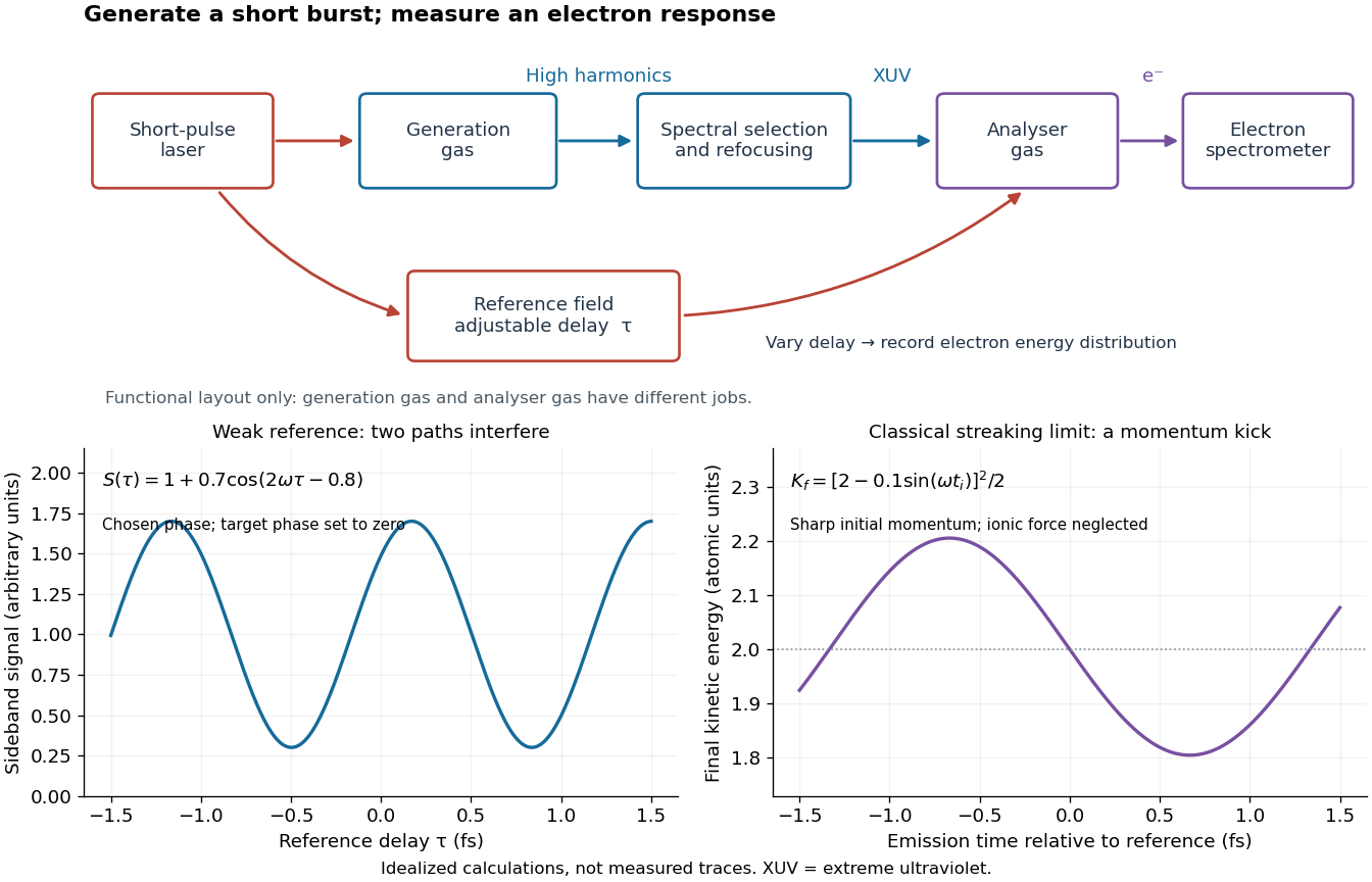
Attosecond physics resolves changes on the scale of seconds, especially electron dynamics. Its central trick is to convert a short optical event into an experimentally accessible energy or phase change. A broad optical spectrum provides the ingredients for a short optical pulse; their spectral phases determine when those ingredients add constructively. High harmonic generation supplies the optical spectrum, while RABBITT and attosecond streaking supply complementary timing measurements. XUV denotes extreme ultraviolet radiation.
There are two separate timing problems: characterize the incident optical pulse, then infer the response of the target. A photoelectron measurement mixes the incident spectral phase, the target's transition response and the probing electric field. Recovering one requires constraints on the others. These methods measure distributions of photoelectron energies over repeated shots, rather than photographing a moving atomic orbital.
Chirped pulse amplification increases an optical pulse's energy while keeping its peak power lower during amplification: stretch the pulse, amplify it, then compress it. A chirp is a changing instantaneous frequency. Stretching separates the arrival times of different frequencies; pulse compression brings their contributions back together. The gain medium supplies energy, whereas the compressor concentrates the surviving energy into a shorter time.
Donna Strickland and Gérard Mourou demonstrated chirped pulse amplification at Rochester in 1985. Their experiment used an optical fiber, a regenerative amplifier and a diffraction grating compressor.[ref]
Compression of amplified chirped optical pulses by Donna Strickland and Gérard Mourou. Strickland and Mourou, corrected December 1985 paper, pp.219–221
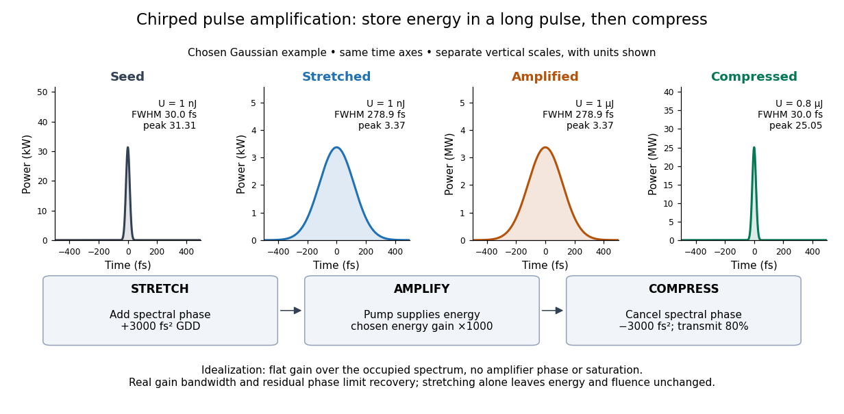
The useful idea is to arrange where the large peak power occurs. Lower light intensity in the amplifier reduces unwanted self-focusing and self-phase modulation; the compressed output can still drive strong nonlinear optics. Stretching does not remove every damage mechanism, and compression does not manufacture energy.
An optical frequency comb has evenly spaced optical spectral lines, or teeth. A mode-locked laser supplies short optical pulses at repetition frequency , the tooth spacing. The carrier-envelope offset frequency positions the whole ruler:Only teeth within the emitted optical spectrum are present; the extrapolated intercept need not be an emitted tooth.[ref]
Passion for Precision by Theodor W. Hänsch. Passion for Precision, p.157: tooth relation
The achievement associated with John L. Hall and Theodor W. Hänsch is a practical bridge between optical frequencies and countable electronic frequencies. Instead of constructing a separate chain of lasers for each optical measurement, a broad comb supplies many linked reference teeth. Stable lasers, short optical pulses and strong nonlinear optics in optical fibers came together around 1999–2000.[ref]
Nobel Lecture: Defining and measuring optical frequencies by John L. Hall. Nobel Lecture: Defining and measuring optical frequencies, pp.1288–1291: chains and comb development
A three-level laser pumps emitters out of their ground state into a higher pump state, which rapidly relaxes into the upper lasing state. The lower lasing state is the ground state itself. Photon absorption on the lasing transition therefore competes with stimulated emission until enough emitters have been removed from the ground state. This is the ground state depletion problem implicit in population inversion.
The model below treats nondegenerate lasing energy levels with equal absorption and emission cross-sections. Its inversion condition is . Real materials require the relevant sublevel populations, degeneracies and transition strengths; the simple half-population condition should not be imposed on every optical transition. Extra levels let the pump and the emitted light act on different transitions, avoiding the steady two-level saturation limit discussed in population inversion.
A laser whose gain medium contains dye molecules. Its tunable wavelength permits laser spectroscopy of different spectral lines.
A semiconductor laser uses a semiconductor as its laser gain medium. Pumping produces carrier populations that permit stimulated emission between suitable electronic states. An optical resonator supplies feedback, and oscillation begins when the gain compensates round-trip losses.
A laser diode supplies pumping by electrical injection; other semiconductor lasers can be optically pumped. The band gap, confinement and resonator determine the possible emission range. A measurement of optical output versus pump strength helps locate the laser threshold, while an emission spectrum tests the modes involved. Increasing output alone does not establish that the device has entered coherent laser oscillation.
The Compact Muon Solenoid is a general-purpose particle detector at the Large Hadron Collider, commonly called the CMS experiment. Its superconducting solenoid surrounds central tracking and calorimeter systems; outer muon detectors work with the magnet's return structure.[ref]
The CMS Experiment by CMS Collaboration. Overview of detector layers and solenoidal magnetic configuration
Charged-particle bending constrains momentum, while electromagnetic and hadronic calorimeters measure deposited energy. Combining tracker, calorimeter and muon information identifies candidate collision products. Agreement among these measurements is more informative than any one image or signal; trigger selection and reconstruction efficiency must also be accounted for when inferring a production rate.
The ATLAS experiment is a general-purpose particle detector at the Large Hadron Collider. Layers around the collision point combine track reconstruction, electromagnetic and hadronic calorimeters, and outer muon detectors. A central solenoid and larger toroidal magnet system provide magnetic bending in different detector regions.[ref]
A charged track's curvature estimates momentum; a calorimeter measures deposited energy; outer signals help identify penetrating muons. Combining these measurements distinguishes candidate particle types and reconstructs decays. Apparent missing transverse momentum is an event balance inferred from the measured products, so detector coverage, calibration and reconstruction errors also affect it.
For a two-dimensional electron gas in a perpendicular magnetic field of magnitude , the filling factor is the electron number per unit area divided by the orbital degeneracy per unit area of one spin branch of a Landau level. Here is the positive elementary charge and the Planck constant. The nominal filling factor varies continuously with ; it need not be an integer.
For an electron in a uniform perpendicular magnetic field of magnitude , the magnetic length sets the orbital length scale of a Landau level; is the positive elementary charge.
For a semiclassical closed electron orbit in a plane perpendicular to a uniform magnetic field, its wavevector-space area obeys . An ordinary parabolic band without an extra geometric phase has . The semiclassical equations rotate and scale the real-space orbit by , giving . For a parabolic band this is equivalent to .
Pinned article: Introduction to the OurBigBook Project
Welcome to the OurBigBook Project! Our goal is to create the perfect publishing platform for STEM subjects, and get university-level students to write the best free STEM tutorials ever.
Everyone is welcome to create an account and play with the site: ourbigbook.com/go/register. We belive that students themselves can write amazing tutorials, but teachers are welcome too. You can write about anything you want, it doesn't have to be STEM or even educational. Silly test content is very welcome and you won't be penalized in any way. Just keep it legal!
Intro to OurBigBook
. Source. We have two killer features:
- topics: topics group articles by different users with the same title, e.g. here is the topic for the "Fundamental Theorem of Calculus" ourbigbook.com/go/topic/fundamental-theorem-of-calculusArticles of different users are sorted by upvote within each article page. This feature is a bit like:
- a Wikipedia where each user can have their own version of each article
- a Q&A website like Stack Overflow, where multiple people can give their views on a given topic, and the best ones are sorted by upvote. Except you don't need to wait for someone to ask first, and any topic goes, no matter how narrow or broad
This feature makes it possible for readers to find better explanations of any topic created by other writers. And it allows writers to create an explanation in a place that readers might actually find it.
Figure 1. Screenshot of the "Derivative" topic page. View it live at: ourbigbook.com/go/topic/derivativeVideo 2. OurBigBook Web topics demo. Source. - local editing: you can store all your personal knowledge base content locally in a plaintext markup format that can be edited locally and published either:This way you can be sure that even if OurBigBook.com were to go down one day (which we have no plans to do as it is quite cheap to host!), your content will still be perfectly readable as a static site.
- to OurBigBook.com to get awesome multi-user features like topics and likes
- as HTML files to a static website, which you can host yourself for free on many external providers like GitHub Pages, and remain in full control

Figure 2. You can publish local OurBigBook lightweight markup files to either OurBigBook.com or as a static website.
Figure 3. Visual Studio Code extension installation.
Figure 5. . You can also edit articles on the Web editor without installing anything locally. Video 3. Edit locally and publish demo. Source. This shows editing OurBigBook Markup and publishing it using the Visual Studio Code extension. 
- Infinitely deep tables of contents:




All our software is open source and hosted at: github.com/ourbigbook/ourbigbook
Further documentation can be found at: docs.ourbigbook.com
Feel free to reach our to us for any help or suggestions: docs.ourbigbook.com/#contact