A family $\mathcal{A}\subseteq [\mathbb{N}{]}^{\omega }$ is Ramsey in the homogeneous-cone sense if there is an infinite $M\subseteq \mathbb{N}$ such that either $[M{]}^{\omega }\subseteq \mathcal{A}$ or $[M{]}^{\omega }\cap \mathcal{A}=\varnothing$. This is the existence of one infinite homogeneous cone. Requiring such a refinement inside every infinite initial ground set gives the stronger definition used for a Ramsey set of infinite subsets; requiring a homogeneous refinement in every finite-stem neighbourhood gives a completely Ramsey set.

These quantifiers should be distinguished. For example, the existence of a homogeneous cone on the even numbers does not constrain a family's restriction to the odd numbers. If $\mathcal{E}$ is the finite-symmetric-difference parity colouring class on the odd numbers, the family consisting of $\mathcal{E}$ alone has a homogeneous cone disjoint from it on the even numbers, but no homogeneous cone on the odd numbers. Every open set in the ordinary topology on infinite subsets has homogeneous cones inside all infinite ground sets, as follows by deciding finite stems through fusion.

A finite stem is a finite initial segment $s$ of an infinite subset of $\mathbb{N}$. The associated neighbourhood in the ordinary topology on infinite subsets is $[s]=\{X:s\text{ is an initial segment of }X\}$. For an infinite tail $A$ above $\max s$, the neighbourhood $[s,A]=\{s\cup B:B\in [A{]}^{\omega }\}$ is basic in the Ellentuck topology. Finite stems allow a fusion argument to fix initial choices while successively thinning the remaining infinite tail.

An algorithm uses polynomial space if its working memory is bounded by a fixed polynomial in the input length. Exponentially many possibilities can still be searched when each candidate and the search counter need polynomial space and storage is reused. The decision problems with deterministic polynomial-space algorithms form PSPACE.

In a nonzero steady one-dimensional flow with an isothermal equation of state with $p=c_s^2\rho$ and constant cross section, the continuity equation gives $\rho u=\text{constant}$. Eliminating density from momentum gives $(u-c_s^2/u)u^{\prime }=-{\Phi }^{\prime }$. With Mach number $\mathcal{M}=|u|/c_s$, integration yields ${\mathcal{M}}^2/2-\ln \mathcal{M}+\Phi /c_s^2=C$. The function $f(\mathcal{M})={\mathcal{M}}^2/2-\ln \mathcal{M}$ has minimum $1/2$ at $\mathcal{M}=1$, so a smooth transonic crossing at $x_{\ast }$ requires a local maximum of $\Phi$ and $C=1/2+\Phi (x_{\ast })/c_s^2$. At a nondegenerate maximum, $f=1/2+(\mathcal{M}-1{)}^2+\cdots$ gives ${\mathcal{M}}^{\prime }(x_{\ast })=\pm \sqrt{-{\Phi }^{\prime \prime }(x_{\ast })/(2c_s^2)}$.

A finitely generated abelian group whose elements all have finite order is finite. Induct on derived length for a finitely generated soluble group with this property. Its abelianization is finite, so its commutator subgroup has finite index and is finitely generated by Schreier's lemma. That subgroup is soluble of smaller derived length and is still a torsion group, hence finite by induction. The ambient group is a finite extension of it and is finite.

A finite group is supersolvable if it has a normal series of a group whose nontrivial factors are cyclic of prime order. This is stronger than solubility, because the individual terms must be normal in the ambient group. For instance, $A_4$ is soluble via its normal Klein four-group, but is not supersolvable: it has no normal subgroup of order two or three with which such a series could begin.

Solvation is stabilization through interactions between a solute and its solvent. It involves both the solute's surroundings and reorganization of the solvent: neighbors move, orientations change, and existing interactions compete with new ones. Electric forces, Van der Waals forces, and specific interactions such as hydrogen bonds can contribute. Solvation can also occur at groups on an insoluble material, so it does not require complete dissolution.^[ref]

Solvation by water is called hydration. Hydration of ions is the charged special case, but neutral molecules such as sucrose can also interact with water without becoming ions. A hydrated cation retains its positive net electric charge; orienting neutral water molecules around it does not supply an extra electron. Dissolution, desolvation, and ionization describe different changes, as the examples below show.^[ref][ref]

The useful question is therefore not just whether a solute attracts a solvent, but how much the whole system gains after paying for the rearrangements. Solvation free energy describes a specified transfer into a solvent; solvation thermodynamic balance explains why even cooling during dissolution can accompany favorable mixing. The existing solubility discussion concerns how much remains dissolved at chemical equilibrium.

An irregular solid harmonic is harmonic on punctured three-dimensional Euclidean space and generally singular at the origin. The Kelvin transform maps a degree-$n$ regular solid harmonic to a constant multiple of its irregular counterpart.

For a long vacuum-core or air-core solenoid with fixed geometry and linear magnetic response, neglecting end effects gives self-inductanceHere $N$ is the total number of turns, $n=N/\ell$ is the solenoid turn density, and $A$ is the interior cross-sectional area. The reason for the square of $N$ is physical: more turns produce more magnetic field, and more turns link the resulting magnetic flux. Approximately equal magnetic flux $\Phi \approx BA$ through each turn gives magnetic flux linkage $\Lambda \approx N\Phi \approx {\mu }_0{N}^{2}AI/\ell$; division by the electric current yields $L$. ^[ref].

For the same $N=1000$, $\ell =0.50\mathrm{m}$, and $a=0.025\mathrm{m}$, the area is $A=\pi (0.025{)}^2{\mathrm{m}}^2\approx 1.9635\times 10^{-3}{\mathrm{m}}^2$. The long-coil estimate isAt $I=0.50\mathrm{A}$, each turn links approximately $2.4674\times 10^{-6}\mathrm{Wb}$ and the total magnetic flux linkage is approximately $2.4674\times 10^{-3}\mathrm{Wb}$. Their ratio to $I$ is the stated self-inductance. A real finite coil need not give precisely these values: the axial centre correction above is not by itself a correction formula for inductance, which depends on magnetic flux across all the turns.

At fixed $A$ and $\ell$, doubling $N$ quadruples $L$. At fixed solenoid turn density $n$ and area $A$, doubling $\ell$ doubles both $N$ and $L$. These are different changes to the geometry, so there is no contradiction between $L\propto 1/\ell$ at fixed $N$ and $L\propto \ell$ at fixed $n$. A magnetic core requires its own magnetic permeability model; nonlinear magnetization can make a constant-$L$ description inadequate.

Model a finite solenoid as a continuum of coaxial turns shaped as circles of radius $a>0$, uniformly distributed over length $\ell$ with solenoid turn density $n=N/\ell$. Put its centre at $z=0$, so its ends are $z=\pm \ell /2$. With the same electric current orientation as in the long-solenoid approximation, its axial magnetic field isThis formula applies only on the axis, where symmetry cancels the transverse magnetic field. It does not describe points off the axis. It is exact for the continuum circular-turn model, which neglects winding thickness, discrete wire spacing, and helical advance. ^[ref].

The derivation is an especially direct use of the superposition principle. The on-axis magnetic field of a circular current loop at source position $z^{\prime }$ is ${\mu }_{0}I{a}^2/[2(a^2+(z-z^{\prime }{)}^2{)}^{3/2}]$. There are $nd{z}^{\prime }$ turns in an axial slice, soSubstitute $u=z-z^{\prime }$ and use the antiderivative $u/[a^2\sqrt{a^2+u^2}]$ to obtain the displayed expression. If the centre is instead at $z=z_0$, replace every $z$ in that expression by $z-z_0$.

At the centre and at either end, respectively,For aspect ratios $\ell /a=2,6,20$, the centre ratios are approximately $0.7071,0.9487,0.9950$. The end ratio tends to $1/2$ as $\ell /a$ becomes large, even though the centre ratio tends to $1$. Thus a long coil can have an excellent central magnetic field while the ends still differ strongly from that value. Convergence to the long-solenoid approximation is not uniform across the end region.

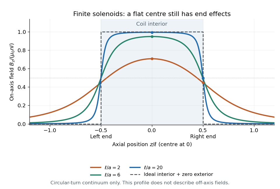
For a concrete geometry, give the earlier coil radius $a=0.025\mathrm{m}$, so $\ell /a=20$. Its central magnetic field is approximately $1.2504\mathrm{mT}$, its end value is $0.6275\mathrm{mT}$, and at $z=\ell$ its axial magnetic field is still $0.00277\mathrm{mT}$. The last point is outside the coil: finite length does not permit the zero-exterior conclusion of the infinite model. Off the axis, the magnetic field lines bend around to form the return field. A central axial value alone also does not determine the total magnetic flux through every turn of a short coil.

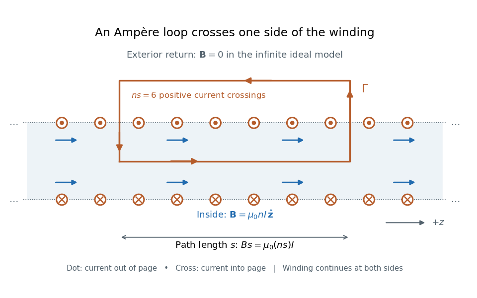
In magnetostatics, an ideal infinitely long solenoid is a cylindrical sheet of circumferential surface current density $K=nI$. It has negligible winding advance, no magnetic core, and no imposed external magnetic field. Choose positive electric current to produce magnetic field along $+z$. In this ideal model the interior magnetic field is uniform and axial, $B={\mu }_{0}nI$, and the exterior magnetic field is zero; ${\mu }_0$ is the vacuum permeability. For a finite, closely wound air-core coil, the same result is an approximation well inside the coil, several radii from either end. Air is treated as having the magnetic permeability of vacuum. ^[ref].

For a short proof, the translational and rotational symmetries of the ideal cylindrical current sheet, together with the Biot-Savart law, give an axial magnetic field. Ampère's law on rectangles wholly outside makes that axial exterior value independent of radius; the condition of no imposed magnetic field makes it zero at infinity and hence everywhere outside. Rectangles wholly inside similarly show that the interior value is independent of radius. Now choose an Amperian loop with axial length $s$, one long side inside and the other outside. The transverse sides are perpendicular to the magnetic field, so their contributions to the line integral vanish. The loop crosses $ns$ turns of the winding, givingHere $s$ is the integration-path length, not the whole coil length $\ell$. An Amperian loop surrounding both sides of the winding encloses equal and opposite electric currents; zero net circulation alone would not prove zero magnetic field at every exterior point.

For the $1000$-turn, $0.50\mathrm{m}$ coil with electric current $I=0.50\mathrm{A}$, the long-solenoid approximation givesThis illustrative calculation uses vacuum permeability ${\mu }_0\approx 1.256637\times 10^{-6}H/m$, a rounded value, not an exact constant. Since the 2019 redefinition of SI, vacuum permeability is determined experimentally.^[ref] Doubling $I$ doubles the ideal magnetic field; doubling $N$ at fixed $\ell$ does the same. Increasing $\ell$ while keeping $N$ fixed decreases $n$ and hence the ideal magnetic field.

The solenoid turn density $n$ counts turns per unit axial length in a uniformly wound solenoid. The total turn count $N$ is dimensionless, whereas $n$ has units ${\mathrm{m}}^{-1}$. A $1000$-turn coil of length $0.50\mathrm{m}$ has $n=2000{\mathrm{m}}^{-1}$; an axial interval of length $s=0.010\mathrm{m}$ then contains $ns=20$ turns. The effective circumferential surface current density in the closely spaced circular-turn model is $K=nI$, with units $A/m$. ^[ref].

For a single-layer helix, the axial advance per turn is approximately $1/n$. The circular-turn model neglects this advance and the associated axial component of electric current, as well as the detailed magnetic field close to individual wires. The number of turns around the whole coil is always $N=n\ell$ here; it must not be substituted for $n$ in $B={\mu }_{0}nI$.

Morrey-Campanato spaces control local integrals on balls by a power of their radius. The Morrey form uses ${\sup }_{x,r}{r}^{-\lambda }{\int }_{B_r(x)}|u{|}^p$; the Campanato space uses $|u-u_{B_r(x)}{|}^p$ instead. Mean subtraction measures oscillation and relates this family to Hölder spaces.

Ladyzhenskaya's inequality controls the Lp norm of a function by its Lp norm and the Lp norm of its gradient: in dimension two, $\Vert u{\Vert }_4\le C\Vert u{\Vert }_2^{1/2}\Vert \nabla u{\Vert }_2^{1/2}$; in dimension three the exponents are $1/4$ and $3/4$. These estimates hold for smooth compactly supported functions and extend using density of smooth functions in a Sobolev space.

A domain has the uniform interior cone property if fixed-height, fixed-opening cones can be placed inside the domain at its points, with an allowed orientation depending on the point. This geometric regularity permits the Sobolev embedding theorem and Rellich-Kondrachov compactness theorem. It is an interior condition, distinct from the exterior cone condition used in boundary regularity.

For $a<b$ and $0\le \theta \le 1$, the displayed estimate holds on Euclidean space and a torus with the Fourier definition of the Sobolev norm. In the squared norm, write the weighted squared Fourier coefficient as the product of its weight-$a$ value to the power $1-\theta$ and its weight-$b$ value to the power $\theta$. Holder inequality then proves the estimate. On a compact manifold, a finite coordinate cover and a partition of unity give the same estimate up to a constant. Young inequality implies the useful absorption form $\Vert u{\Vert }_{H^{s+1}}\le \epsilon \Vert u{\Vert }_{H^{s+2}}+C_{s,\epsilon }\Vert u{\Vert }_2$ for nonnegative $s$.

On a bounded Lipschitz domain, the Sobolev trace operator is the continuous linear extension to $H^1(\Omega )$ of the boundary restriction of smooth functions. Continuity and density make this extension unique; its existence is the Sobolev trace theorem. The kernel prescribes a homogeneous Dirichlet boundary condition. Vanishing Sobolev trace on only part of the boundary instead gives the form domain for a mixed boundary condition, with the natural Neumann boundary condition on the remainder. On an assembly of congruent tiles, taking a Sobolev trace commutes with a constant matrix acting on the tile restrictions. This lets a transplantation theorem be proved on quadratic form domains even when corner eigenfunctions have singular classical derivatives.

For matrix-valued circle loops in $H^s$, $s>1/2$, use a submultiplicative algebra norm with contractive Fourier projections. If $\Vert X-I\Vert <1$, solve $Y_{+}=I+y_{+}$ by $y_{+}=-P_{>0}((X-I)(I+y_{+}))$, and solve $V_{-}=I+v_{-}$ by $v_{-}=-P_{<0}((I+v_{-})(X-I))$. Both are contractions. Then $X{Y}_{+}$ has only nonpositive modes, $V_{-}X$ has only nonnegative modes, and their compatible products equal a constant matrix. Invertibility of the Hardy compression $I+P_{\ge 0}(X-I)$ makes that constant invertible. This yields the stated normalized factors; uniqueness follows because the two Fourier subalgebras intersect in constants.

The zero-trace first-order Sobolev space is the closure of $C_c^{\infty }(\Omega )$ in the $H^1$ norm. On a bounded Lipschitz domain it is the kernel of the Sobolev trace operator. On an interval, its elements have absolutely continuous representatives with both endpoint values zero. The Poincaré inequality makes the derivative norm equivalent to the full Sobolev norm. This is the natural form domain for an elliptic problem with homogeneous Dirichlet boundary conditions.

The displayed surfaces, with positive semiaxes, are hyperboloids. The plus sign gives a one-sheet hyperboloid, while the minus sign gives a two-sheeted hyperboloid.