Two closed oriented rational Witt spaces are Witt bordant if their signed disjoint union is the collared boundary of a compact oriented Witt space with collared boundary. Disjoint union gives the bordism group ${\Omega }_n^{\mathrm{Witt}}$.

Measurement-based quantum feedback adapts a control input from a measurement record or conditional quantum state estimate. A measurement contributes backaction and generally stochastic dynamics. Exact instantaneous expectation values cannot be read from a single system without these effects. A feedback law derived for deterministic closed-system evolution therefore needs a new conditional dynamical analysis before being applied as measurement feedback.

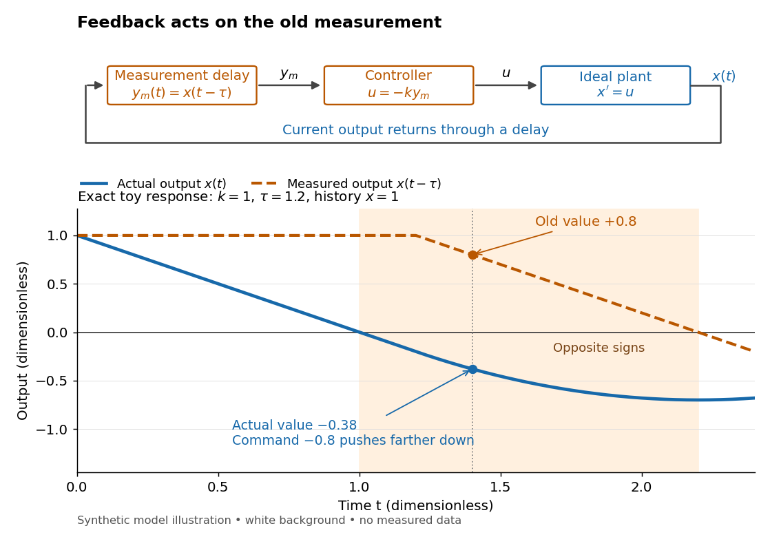
A feedback delay means a controller reacts to an earlier plant output. An accurate measurement can still be stale: when the plant output has already crossed the reference signal, a controller using the earlier value may continue pushing it away from the target. In a pure constant-delay model, $y_m(t)=y(t-\tau )$ with $\tau \ge 0$. This isolates timing from measurement noise; it does not describe every sampling or communication mechanism. ^[ref]

For the ideal scalar controlled plant $\dot{x}=u$, a zero reference signal, no control disturbance, and proportional control with constant feedback gain $k>0$, the equations areWith $\tau =0$, this is an ordinary differential equation with exponential decay $x(t)=x(0)e^{-kt}$. With $\tau >0$, it is a delay differential equation, requiring an initial history of delayed feedback. The delay stability of proportional integrator control depends on the product $k\tau$: even this simple controlled plant loses asymptotic stability at $k\tau =\pi /2$.

Integral action adds memory of the tracking error to a controller: $z(t)=z(0)+{\int }_0^{t}e(s)ds$. A persistent tracking error keeps changing $z$, so an equilibrium point with constant $z$ must have $e=0$. The accumulated value can remain nonzero after the tracking error has vanished, maintaining the control input needed to cancel a constant control disturbance. Convergence still requires a stable feedback control design. ^[ref]

Proportional control chooses a control input proportional to the current tracking error. For the ideal controlled plant and constant reference signal $r$, its ordinary differential equation is $\dot{x}=k(r-x)+w$. With $w=0$ and initial condition $x(0)=x_0$, the exact response isFor $r=1$, $x_0=0$ and $k=2$, this gives $x(1)=1-e^{-2}\simeq 0.864665$ and $x(2)=1-e^{-4}\simeq 0.981684$. To verify the formula, substitute it into the ordinary differential equation and check the initial condition; its decaying exponential function explains the approach to the goal.

With a constant control disturbance, setting $\dot{x}=0$ gives the equilibrium point $x_{\ast }=r+w/k$ and steady-state tracking error $e_{\ast }=-w/k$. For $w=0.2$, doubling the feedback gain from $k=2$ to $k=4$ reduces the offset from $0.1$ to $0.05$. This improvement is a statement about the ideal model: it neglects feedback delay and measurement noise, so it does not establish that arbitrarily large feedback gains are safe. ^[ref]

In the first diagram's switched control disturbance experiment, $k=2$ and $w=0.2$ from $t=2$ give, for $t\ge 2$,Thus $x(4)\simeq 1.097833$ and $x(8)\simeq 1.099999$. At the equilibrium point, the controller supplies $u=-0.2$ to cancel the control disturbance. Proportional control needs a nonzero tracking error to produce that persistent correction.

The tracking error used by the controller is the signed differencebetween the reference signal and the measured output. A positive tracking error means the readout is below the desired value; a negative tracking error means it is above. With exact measurement $y_m=y$, $r=1$ and $y=1.1$ give $e=-0.1$. For a positive-response controlled plant, positive feedback gain in proportional control $u=k_{p}e$ then reduces the plant output. The sign of the controller must also account for the sign of the controlled plant's response: a positive command that reduces the plant output requires a different sign choice. Kantor uses the opposite tracking error convention, $PV-SP$, together with a minus sign in his controller; translating both signs gives the convention here. ^[ref]

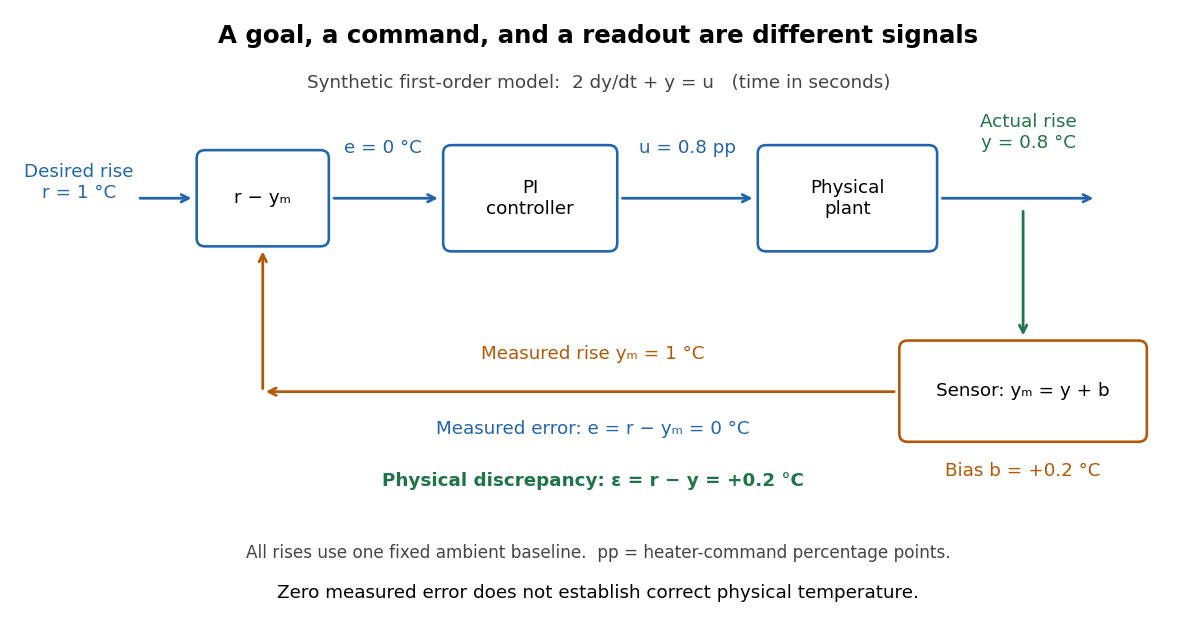
Distinguish the controller's tracking error from the physical plant output discrepancy $\epsilon =r-y$. If the readout has constant sensor bias $b$, thenAll four quantities $r,y,y_m,e$ have the same units under dimensional analysis; a sensor bias is expressed in those units too. A readout that is too high by $0.2{}^{\circ }\mathrm{C}$ can make $e=0$ when the physical temperature is $0.2{}^{\circ }\mathrm{C}$ below the goal. Integral action integrates the tracking error it receives; it cannot infer this missing calibration information from that tracking error alone. Thermometer calibration against an independent reference addresses a different problem from tuning a feedback gain.

A motivating apparatus/model comparison is Park, Martin, Kelly and Hedengren's temperature-control laboratory: two TIP31C heaters with attached TMP36GZ sensors and heat sinks, an Arduino, a power supply, and a USB-connected computer. The readout converts sensor voltage to temperature; software records that measured output while specifying heater commands from $0$ to $100\%$. For the single-heater test, one command changes in steps and the other heater stays off. Parameters are fitted to one run, then a different command sequence tests predictions without feeding measured temperatures into the simulation. The authors observe that their richer thermal model predicts the response better than the approximation with a single time constant and a delayed control input, especially after command changes. The real sensor has its own thermal lag. They also repeat the same command profile at different ambient temperatures and find changes in the response, motivating ambient-condition reporting. This experiment measures a command-to-readout response, not independently the exact heater temperature or delivered power. ^[ref]

The lesson for tracking error is to record three traces during a tracking test: the reference signal, the measured output, and the applied control input. Their first difference is the tracking error; a model prediction minus a readout is instead a model discrepancy. In a proposed comparison of proportional control and proportional-integral control, keep the initial temperature, ambient conditions, heater limits, and target changes fixed; run the second heater separately as a known control disturbance. Independent thermometer calibration is needed to assess physical accuracy. These are suggested controls, not additional experiments claimed for the paper. A sensor's lag, measurement noise, actuator saturation, and changed ambient conditions can all invalidate conclusions drawn from the ideal first-order model.

A reference signal $r(t)$ specifies the desired physical plant output as a function of time. A fixed reference signal is often called a setpoint; a changing reference signal describes a trajectory to follow. A reference signal is a goal, whereas the control input $u(t)$ is the command chosen to achieve that goal. ^[ref]

Asking for a temperature of $40{}^{\circ }\mathrm{C}$ does not specify a heater command of $40\%$: dimensional analysis distinguishes the units of these quantities. The reference signal and the measured output must describe the same quantity in the same coordinates before their difference can define a tracking error. An unconverted sensor readout cannot be subtracted directly from a desired temperature.

For example, let $y=T-T_0$ be temperature rise above a fixed ambient baseline $T_0$, and write the desired temperature as $T_d=T_0+r$. A Heaviside step function gives $r(t)=R$ for $t\ge 0$, with $r(t)=0$ before the change: the target rise becomes $R$ at once, although a physical controlled plant generally cannot jump at once. A ramp reference signal $r(t)=vt$ instead asks the temperature rise to increase at a fixed rate $v$. If $R=1{}^{\circ }\mathrm{C}$ and $v=0.2{}^{\circ }\mathrm{C}{\mathrm{s}}^{-1}$, the first reference signal asks for a lasting one-degree rise; the second asks for a one-degree rise at $t=5\mathrm{s}$ and a two-degree rise at $t=10\mathrm{s}$. Here degree Celsius differences are also kelvin differences. A target that grows forever is useful for analytical tests but eventually exceeds a real heater's range.

To make the distinction between a goal and a command concrete, the examples in steady-state tracking error use the first-order low-pass filter as a new controlled plant, rather than the accumulating controlled plant $\dot{x}=u+w$ used in the earlier feedback demonstration:The time constant $\tau$ has units of time, $K$ has units of plant output per control input, and the additive control disturbance $d$ has the units of $y$. This $d$ is an equivalent output offset, not the rate-like $w$ in $\dot{x}=u+w$. A heater interpretation uses $y$ in degree Celsius differences and $u$ in percentage points of heater command, with $K$ in degrees per percentage point; the control input is a command, not a direct measurement of delivered power. With exact measurement, holding $y=R$ requires $u=(R-d)/K$. Thus even a constant reference signal can require a persistent nonzero control input. The numerical model below is deliberately synthetic and has no fitted laboratory parameters.

Snowflake yeast are cluster-forming Saccharomyces cerevisiae with branching connections between mothers and attached daughter biological cells. They provide an experimental system for studying early transitions to simple multicellular organisms; see the protocol, observations and limits under multicellular organism.

A clinical trial comparison must define a common time origin and observation window for both assigned treatments. A probability measured from allocation cannot be replaced by one measured from a later treatment-dependent release or discharge. The latter may describe a different time interval and a selected population. A numerical sample size cannot be obtained by silently treating those probabilities as interchangeable.

Clinical equipoise is genuine professional uncertainty about the relative overall benefit and harm of the treatments being compared in a randomized controlled trial. A favorable intermediate endpoint does not by itself resolve uncertainty about mortality. Ethical design requires informed consent, meaningful benefit-risk assessment and monitoring of serious harms; an underpowered safety comparison is not evidence that harm is absent.

Independent trial safety monitoring reviews accumulating serious outcomes according to a prespecified plan and may recommend stopping or modifying a clinical trial when harm or benefit changes the ethical balance. Complete ascertainment of deaths and other severe outcomes is needed even if the trial is sized for a different endpoint. Pooled evidence and prespecified sequential thresholds can make rare-event monitoring useful without presenting a nonsignificant harm comparison as safety.

Radiative forcing is a change in the net downward radiative flux caused by an imposed perturbation, evaluated with a specified adjustment convention before the surface climate responds. State the reference period and whether the diagnostic is at the tropopause or top of the atmosphere. A local seasonal ocean heat flux is not directly interchangeable with global annual radiative forcing.

The Arctic dipole anomaly describes a pressure pattern with opposed anomalies on the North American and Eurasian sides of the Arctic. It is distinct from the more nearly annular Arctic Oscillation; associated winds can change sea ice export and warm-air advection.

Global mean sea level can rise through changes in ocean volume at fixed mass and through additions of ocean mass. Local relative sea level additionally depends on ocean circulation, gravity and vertical motion of the land. Floating sea ice has already displaced seawater, so its melt has a much smaller direct sea-level effect than transfer of grounded land ice into the ocean.

Global warming is an increase in Earth's global mean surface temperature. It is one aspect of climate change, which also includes changes in precipitation, circulation, extremes and the cryosphere. Warming driven by additional greenhouse gases can be amplified or moderated by climate feedbacks.

Attribution of recent climate change assesses the contributions of anthropogenic forcing, natural forcing and internal variability to observed changes. It combines the physics of radiative transfer, measured forcing agents, energy budgets and spatial, vertical and temporal response patterns. A single weather event or a single trend is insufficient by itself to identify all causes.

Polar amplification is greater temperature change at high latitudes than in the global mean. Ice-albedo feedback, the vertical structure of atmospheric warming, the temperature dependence of radiative cooling, ocean heat storage, clouds and energy transport all contribute; the balance differs between the Arctic and Antarctic and between seasons.

Derrick's scaling argument tests whether a static localized field configuration can be an energy extremum under a change of size. For ${\varphi }_{\lambda }(x)=\varphi (\lambda x)$ in $D$ spatial dimensions, a term homogeneous in $m$ spatial derivatives scales as $E_m(\lambda )={\lambda }^{m-D}{E}_m$.

Stationarity requires ${\sum }_m(m-D)E_m=0$. Nonzero scaling contributions must balance, while terms with $m=D$ have zero scaling weight and need no opposite-power partner. This qualification matters for scale-invariant two-dimensional gradient models. In an unconstrained scalar model with positive ordinary gradient and potential energies in more than two dimensions, both scale in the same direction, obstructing a nontrivial static finite-energy minimum. Higher derivatives, gauge fields, constraints, time dependence or conserved-charge conditions can change the argument. The scaling identity is necessary, not a complete proof of stability.

A non-topological soliton is a localized finite-energy field configuration whose existence or stability is not protected by a nontrivial topological charge. A conserved ordinary Noether charge can instead obstruct its decay. A Q-ball is a standard complex-scalar example: its profile is localized while its phase rotates in time.

Lagrangian field theory specifies an action by integrating a Lagrangian density $\mathcal{L}(\varphi ,\partial \varphi ,x)$ over spacetime. Requiring its first variation to vanish for compactly supported field variations yields the field Euler-Lagrange equations. The variational Lagrangian is the integrand, whereas this field-theoretic formalism specifies the continuum fields and their dynamics.