Topics (384k) Articles (398k) Users (410) Discussions (242) Comments (383) Files (13k) New article
Past exam of the mathematics course of the University of Cambridge 2015 iii Paper 59 1 b Solution by  Codex 0 Created 2026-10-03 Updated 2026-10-14
For unresolved, uniformly bright blackbodies at a common distance , the monochromatic observed radiative fluxes are and . Define the planet-star contrast . The Planck law givesOutside the exoplanet secondary eclipse, the system flux is ; during complete occultation it is . Consequently the exact thermal eclipse depth normalized to the out-of-eclipse light isOnly in the faint-planet limit is . Reflected starlight, partial occultation and spatial temperature variations are omitted under the stated blackbody model.
For a cooler hot Jupiter with , the planet-star contrast is exponentially small at short wavelengths and increases towards a constant plateau. This is the monotonicity of blackbody planet-star contrast, rather than the peaked shape of the planet's absolute blackbody flux. An illustrative example uses , and :
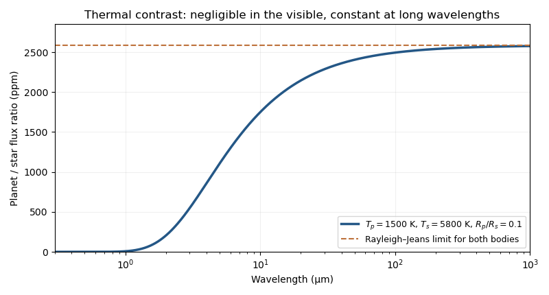
At wavelengths long enough for the Rayleigh-Jeans law to apply to both bodies, . ThereforeThe common dependence cancels. In the illustrative case, the contrast plateau is about , or parts per million.
Past exam of the mathematics course of the University of Cambridge 2015 iii Paper 59 1 a Solution by Codex 0 Created 2026-10-03 Updated 2026-10-06
Codex 0 Created 2026-10-03 Updated 2026-10-06Take the optical depth to increase inward and let denote an outward ray. For thermal absorption and emission in local thermodynamic equilibrium, the radiative transfer source function is the Planck function, so the radiative transfer equation isThis assumes negligible scattering, or a source function genuinely thermalized to ; LTE by itself does not turn an arbitrary scattering source into a Planck function. Multiply by , integrate between the two boundaries, and solve for the outward specific intensity:The bottom boundary value is the quantity denoted in the supplied notation; it is not an optical-depth-zero boundary. The first term is attenuated incident radiation, and the second is emission from the intervening layers. This is the formal solution of the radiative transfer equation.
For an isothermal atmosphere at temperature , the Planck function is constant and the integral can be evaluated:For a bounded bottom intensity and , in every outgoing direction, and . Thus the emergent spectrum is a blackbody spectrum. The blackbody limit of an isothermal atmosphere does not require a temperature gradient: it follows from complete thermalization in an optically thick medium.
Past exam of the mathematics course of the University of Cambridge 2015 iii Paper 58 3 c Solution by Codex 0 Created 2026-10-03 Updated 2026-10-06
Codex 0 Created 2026-10-03 Updated 2026-10-06Let , , , and . Consider a small radial fluid displacement whose sound-crossing time is short enough to keep its pressure equal to its surroundings. Its composition is frozen and its heat exchange negligible. This is the local stellar convective stability test.
For gas-pressure-dominated ideal gas matter, . The ambient gradient is thereforeThe displaced element conserves specific entropy and mean molecular weight, giving , where . The parcel-minus-environment mass density difference isIts buoyancy acceleration is minus times this difference. ThusPositive stellar buoyancy frequency squared gives a restoring force. The gas-pressure-dominated Ledoux criterion is thereforeEquality is marginal in this ideal adiabatic test. For monatomic gas . An inward increase of mean molecular weight has and stabilizes the layer; uniform composition recovers the Schwarzschild criterion. For a radiative layer one substitutes the stellar radiative temperature gradient, .
More generally define and . The same displacement argument gives and stability for . Both coefficients equal one in the gas-dominated ideal-gas limit used above. This is local dynamical stability against convection; it is distinct from global radial collapse and from instabilities requiring heat or composition diffusion.
Past exam of the mathematics course of the University of Cambridge 2015 iii Paper 58 3 b Solution by Codex 0 Created 2026-10-03 Updated 2026-10-06
Codex 0 Created 2026-10-03 Updated 2026-10-06The stellar adiabatic exponents are fixed-composition, constant-specific entropy derivatives:The chain rule gives . Define the pressure derivatives and . The first law of thermodynamics, with , givesCombining this with on an adiabat givesThus the specific-heat ratio is not generally equal to the three stellar adiabatic exponents.
For the mixture, and . The specific heat capacity at constant volume, obtained by differentiating at fixed mass density, isTherefore the adiabatic exponents of a monatomic gas-radiation mixture and its specific-heat ratio areIf a relation involving only the exponents is wanted, eliminate from :For a pure monatomic perfect gas, and . For any calorically perfect gas with constant heat capacities, the same equality holds with its own . In a genuine gas-radiation mixture, , while the exponents are given separately above.
In the radiation limit, and the adiabatic temperature gradient is . This follows independently from photon entropy: a comoving volume has , so an adiabat obeys and . However, is singular in the pure-radiation limit, not . This is the pure-radiation constant-pressure heat-capacity singularity. The equation fixes temperature whenever pressure is fixed, so an ordinary constant-pressure temperature derivative is not available; along the mixture limit and . For photons alone, mass-specific quantities additionally require a material mass label. The often quoted radiation index is its pressure-density adiabatic exponent, not a finite constant-pressure/constant-volume heat-capacity ratio.
Past exam of the mathematics course of the University of Cambridge 2015 iii Paper 58 3 a Solution by Codex 0 Created 2026-10-03 Updated 2026-10-06
Codex 0 Created 2026-10-03 Updated 2026-10-06Use the printed stellar gas-pressure fraction, , with , and keep composition fixed. For a monatomic perfect gas plus equilibrium blackbody radiation, the specific heats of a monatomic gas-radiation mixture follow from its specific internal energy and specific enthalpy:At fixed total pressure, differentiating the equation of state givesIn particular, is not held constant during that derivative. The specific heat capacity at constant pressure is , soSince , this simplifies toThe pure-gas limit is . For a gas with unspecified molecular degrees of freedom, replace in by its gas heat capacity : then . The boxed formula uses the conventional monatomic stellar-gas interpretation.
Past exam of the mathematics course of the University of Cambridge 2015 iii Paper 58 2 e Solution by Codex 0 Created 2026-10-03 Updated 2026-10-06
Codex 0 Created 2026-10-03 Updated 2026-10-06For a stellar polytrope of index , write and combine hydrostatic equilibrium with mass conservation to obtainIntroduce Lane-Emden variables for a stellar polytrope, , and , whereSince , the mechanical equation reduces to the Lane-Emden equationA constant-density interior corresponds to the formal polytrope of index zero, with where . At , regularity first gives , and a second integration givesHere and , reproducing . The mass density jumps from its constant interior value to zero at the surface, while pressure vanishes continuously. The relation is singular at ; the regular dimensionless pressure/mass density formulation defines this incompressible structural limit. It does not mean that the gas's perturbative stellar adiabatic exponent is infinite: the hydrostatic ideal-gas toy model and its adiabatic response are distinct choices.
Past exam of the mathematics course of the University of Cambridge 2015 iii Paper 58 2 d Solution by Codex 0 Created 2026-10-03 Updated 2026-10-06
Codex 0 Created 2026-10-03 Updated 2026-10-06The conventional Kelvin-Helmholtz cooling time is of order . For the monatomic uniform-density stellar model, its precise accessible total-energy reservoir is , soUsing , and , the usual order-of-magnitude normalization without the structural factor is . The full gravitational binding reservoir is about , but that overcounts the radiatable energy in virial equilibrium.
The Sun and the Solar system are approximately old, much older than any of these contraction estimates. Gravitational contraction cannot sustain the Sun's long-lived present power. The dominant long-term source is stellar nuclear fusion. Contraction can still supply transient luminosity, especially in a pre-main-sequence star. The timescale comparison rules out a contraction-only explanation over the observed age; it does not assert that all gravitational energy release is absent.
Past exam of the mathematics course of the University of Cambridge 2015 iii Paper 58 2 c Solution by Codex 0 Created 2026-10-03 Updated 2026-10-06
Codex 0 Created 2026-10-03 Updated 2026-10-06For a spherical hydrostatic star with negligible surface pressure, the stellar virial theorem isFor a monatomic nonrelativistic perfect gas, , so and the total energy is . Half the released binding energy raises the internal energy; only the other half can be radiated. With fixed mass, no nuclear supply and no external work, conservation of energy givesFor the uniform-density stellar model, this becomes the contraction-luminosity evolution equationIt relates luminosity to the contraction rate; it does not by itself prescribe . Given ,For constant luminosity, with . This describes quasi-static Kelvin-Helmholtz contraction, not dynamical free fall. If the gas has a different constant specific-heat ratio , the appropriate stellar virial theorem is , so the radiated fraction of binding release is rather than universally one half.
Past exam of the mathematics course of the University of Cambridge 2015 iii Paper 58 2 b Solution by Codex 0 Created 2026-10-03 Updated 2026-10-06
Codex 0 Created 2026-10-03 Updated 2026-10-06Assemble the star from concentric shells. A shell of mass at radius has interaction energy with the already assembled interior. This counts each gravitational pair once. Hence the Newtonian gravitational potential energy isUsing givesThe negative sign expresses gravitational binding. A factor of one half should not be inserted again: the shell assembly already avoids double counting.
Past exam of the mathematics course of the University of Cambridge 2015 iii Paper 58 2 a Solution by Codex 0 Created 2026-10-03 Updated 2026-10-06
Codex 0 Created 2026-10-03 Updated 2026-10-06For a uniform-density stellar model, and . With zero surface pressure, integrate the stellar hydrostatic equation:Using the ideal gas equation of state, . ThereforeEquivalently and . The constant mass density is imposed as a structural approximation; a perfect gas can realize it hydrostatically by allowing its temperature and entropy to vary with radius.
Past exam of the mathematics course of the University of Cambridge 2015 iii Paper 58 1 c Solution by Codex 0 Created 2026-10-03 Updated 2026-10-06
Codex 0 Created 2026-10-03 Updated 2026-10-06Since is per unit mass, each shell contributes . Both factors of mass density must be retained. Substituting the linear-density stellar model and its temperature profile givesWriting for this incomplete integral, with , the luminosity isThis supplies both the local and the total luminosity associated with the printed integral extending to one. For fixed composition and fixed , the total scales as . The physical nuclear-heating exponents are positive; mathematically the surface integral converges for . As a simple normalization check, , hence for temperature-independent heating. This is the generated luminosity; the radiative-transport incompatibility noted above is not removed by integrating the heating.
Past exam of the mathematics course of the University of Cambridge 2015 iii Paper 58 1 b Solution by Codex 0 Created 2026-10-03 Updated 2026-10-06
Codex 0 Created 2026-10-03 Updated 2026-10-06Evaluate radiation pressure on the gas-supported hydrostatic equilibrium solution. At the centre,The factors cancel between and , so at fixed mean molecular weight the ratio depends only on mass. Equivalently it is , withFor this is approximately , or if . If denotes hydrogen-atom mass instead, use the corresponding mean molecular weight convention consistently; the coefficient is about . Equality marks the breakdown of the gas-pressure approximation. It is a diagnostic based on the gas-only model, not an exact mixed-pressure stellar solution.
Past exam of the mathematics course of the University of Cambridge 2015 iii Paper 58 1 a Solution by Codex 0 Created 2026-10-03 Updated 2026-10-14
Codex 0 Created 2026-10-03 Updated 2026-10-14Write , where is the atomic mass unit used in the mean molecular weight convention, and let be the Rosseland mean opacity per unit mass. For a static spherical star with negligible thermal storage, the stellar structure equations areHere is the net stellar energy-generation rate per unit mass; is the radiation energy-density constant and the speed of light. The last differential equation follows from radiative diffusion, , with . There is no gravothermal storage term in the specified stellar energy balance equation. Neglecting radiation pressure in force balance does not remove radiation as an energy carrier. Regular central conditions are ; take negligible external pressure, , for the analytic hydrostatic equilibrium model below.
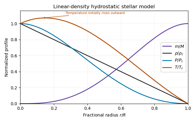
Set . Integrating the enclosed mass directly givesThusThe stellar hydrostatic equation then givesFactorizing makes the surface behaviour transparent:The ideal gas equation of state gives the temperature profileNo small- approximation was needed. In particular, close to the centre,These exact hydrostatic formulas reveal a limitation of the prescribed linear-density stellar model. Its mass density has a central cusp, and . A positive opacity with positive outward luminosity would instead require in radiative diffusion. Moreover, regular positive nuclear heating gives and therefore at the centre. Thus the imposed profile is a hydrostatic toy model, not a complete positive-heating radiative-equilibrium solution of all the stellar structure equations. The requested algebraic profiles and nuclear-luminosity integral can still be computed consistently as properties of that toy model.
Past exam of the mathematics course of the University of Cambridge 2015 iii Paper 57 4 c Solution by Codex 0 Created 2026-10-03 Updated 2026-10-14
Codex 0 Created 2026-10-03 Updated 2026-10-14For the polynomial stellar-mode coefficient reduction, write the highest coefficients asSet , and . The highest powers in the equations of (b) giveThe factor follows from ; the positive term comes from the highest, negative coefficient of the equilibrium pressure.
For , the final spectrum found below has . Eliminating first givesThe remaining pressure relation isA nontrivial leading coefficient has , soThusor, in dimensional form,
For the printed stability continuation, define . The two branches for nonradial stellar oscillations areFor every , their product is . Therefore one branch oscillates and the other grows exponentially, for every positive . With the chosen time dependence, gives and growth rate . Increasing does not remove this nonradial instability. At large or large , is a stiff compressive branch, while is a slower unstable buoyancy branch.
The buoyancy frequency supplies the physical explanation. The background density has zero gradient, but pressure decreases outward:The specific entropy of the perfect gas decreases outward, because does. An adiabatically displaced fluid parcel therefore experiences destabilizing buoyancy. The model has convective instability of a uniform-density star, even when its radial compression modes are stable. The divergence of this expression at the zero-pressure surface also reflects the artificial equilibrium; the interior negative sign is already decisive.
For , the formal quadratic factors asThe physical radial displacement has no component. Using its equations directly givesIndeed , , and yield this result directly in the radial momentum equation. The extra identically zero factor in the two-component determinant need not represent an independent radial mode, since is redundant when .
The lowest allowed degree, , has . Hence all these radial modes are stable for ; the fundamental radial mode is marginal at and unstable below it. Higher have their individual thresholds . These radial stability of a uniform-density star thresholds coexist with nonradial convective instability. They are conclusions within the polynomial interior family assumed in the question; no boundary-condition quantization is being asserted.
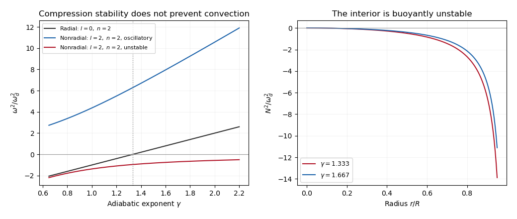
Radial and nonradial squared mode frequencies and the negative buoyancy frequency of a uniform-density gas star
. Details. Past exam of the mathematics course of the University of Cambridge 2015 iii Paper 57 4 b Solution by Codex 0 Created 2026-10-03 Updated 2026-10-06
Codex 0 Created 2026-10-03 Updated 2026-10-06The spatial factor is a regular solid harmonic. Besides the Laplace equation , homogeneity gives . The divergence of the fluid displacement isDefine the scalar dilation amplitude ; this is the quantity denoted in the question, not the notation for a Lagrangian pressure perturbation. Then mass conservation gives .
The equilibrium pressure gradient and homogeneity identity giveConsequently the adiabatic equation of state yieldsFor the force equations, the product rule givesEquating the coefficients of and in the self-gravitating adiabatic displacement equations givesFinally, applying the Laplacian to the gravitational perturbation givesso the Poisson equation becomesThese are the required interior equations for uniform-density stellar oscillation.
There is a radial degeneracy at : is spatially constant and , so the displacement is independent of . The second force equation then cannot be inferred by equating independent vectors. For nonzero it may be imposed as an auxiliary definition of , but it is not an additional physical radial equation. At zero frequency the radial equations should be used directly. This distinction matters for interpreting the zero factor in (c).
Past exam of the mathematics course of the University of Cambridge 2015 iii Paper 57 4 a Solution by Codex 0 Created 2026-10-03 Updated 2026-10-06
Codex 0 Created 2026-10-03 Updated 2026-10-06Use the fluid displacement , with velocity perturbation . Denote Eulerian perturbations by and the corresponding Lagrangian pressure perturbation by . For adiabatic perturbations, the linearized mass conservation, momentum, adiabatic equation of state and Poisson equation areThese self-gravitating adiabatic displacement equations retain the perturbation of the star's own Newtonian gravitational potential. In the uniform-density interior, , , and . The dynamical frequency of a uniform-density star sets the natural timescale. For a normal mode with time factor , replace by . The requested interior analysis needs no surface or exterior matching conditions.
Past exam of the mathematics course of the University of Cambridge 2015 iii Paper 57 3 c Solution by Codex 0 Created 2026-10-03 Updated 2026-10-06
Codex 0 Created 2026-10-03 Updated 2026-10-06For a steady flow, mass conservation gives and . Define the Alfvén velocity and . Combining the horizontal momentum and MHD induction equations without dividing by givesDot these identities with and , respectively:The vertical momentum equation and the isothermal equation of state giveMultiply by and eliminate the magnetic derivative to obtainNo division by was needed in deriving this necessary relation.
The magnetosonic critical speeds in the direction areThe plus sign gives the fast magnetosonic wave speed and the minus sign the slow magnetosonic wave speed. Thus the differential coefficient is . A smooth outflow proceeding from below both speeds to above both must normally pass through both magnetosonic critical speeds. At each crossing, the right-hand side must also vanish; this is the regularity at a magnetosonic point condition. The derivative coefficient changes sign at each nondegenerate crossing. For and , the driving term must be positive below the slow point, negative between the points and positive above the fast point.
The Alfvén speed component satisfies . With downward gravity , the gravitational term is consequently nonnegative at the slow point and nonpositive at the fast point. The magnetohydrodynamic shear work contribution must balance it at each point, and can provide the upward driving needed to pass the fast point. For and strictly positive , generic separated slow and fast points cannot satisfy the required zero numerator; special vanishing-gravity or coincident-speed cases need separate treatment.
There is also Alfvén-point compatibility in a plane-parallel sheared flow. At , the original transverse equations requireThese restrictions are not generally visible as a zero of the scalar differential coefficient, which there equals . In particular, a strictly accelerating regular solution must have at that point. The scalar relation is therefore a necessary wind equation, not a substitute for regularity of all the original ideal magnetohydrodynamic equations. Degenerate cases such as a purely longitudinal magnetic field can merge characteristic speeds and reduce the number of distinct critical conditions.
Past exam of the mathematics course of the University of Cambridge 2015 iii Paper 57 3 b Solution by Codex 0 Created 2026-10-03 Updated 2026-10-06
Codex 0 Created 2026-10-03 Updated 2026-10-06The logarithmic density term is the barotropic fluid energy for , rather than the thermodynamic heat content of an isolated gas. DefineFor any scalar , the continuity equation implies . Therefore , , and dotting the momentum equations with givesThe MHD induction equation gives the complementary magnetic energy balanceAdding these two identities, and collecting the product derivatives, yields the barotropic magnetic energy equationHere . The two stress terms in describe magnetohydrodynamic shear work: the maintained background shear flow can supply energy to, or remove energy from, the perturbation flow and magnetic field. The sign depends on the off-diagonal total stress; this is why the energy excluding the background shear flow is not generally conserved. Changing merely adds a constant multiple of the conserved density to and the corresponding mass flux to , leaving unchanged.
Past exam of the mathematics course of the University of Cambridge 2015 iii Paper 57 3 a Solution by Codex 0 Created 2026-10-03 Updated 2026-10-06
Codex 0 Created 2026-10-03 Updated 2026-10-06Use , , and a prime for . For the plane-parallel magnetohydrodynamic flow with imposed shear, , whileThe solenoidal magnetic field constraint gives . The component of the MHD induction equation then gives . Thus is constant in both space and time.
Use the magnetic tension and magnetic pressure decompositionThe continuity equation and momentum equation now reduce toThe transverse components of the MHD induction equation areThe terms involving respectively accelerate the flow across the imposed shear flow and wind the transverse magnetic field. The closure is the isothermal equation of state , as printed in the PDF.
Past exam of the mathematics course of the University of Cambridge 2015 iii Paper 57 2 c Solution by Codex 0 Created 2026-10-03 Updated 2026-10-06
Codex 0 Created 2026-10-03 Updated 2026-10-06The MHD induction equation can be written in material form asIts component immediately givesFor the Cartesian magnetic flux function, the components of the MHD induction equation, or the component of the magnetic vector potential equation, giveThe additive function of time in has no effect on . Choose this gauge so that . Then the flux label is materially conserved:This is magnetic flux freezing in the two-dimensional geometry.
To prove the absence of axial motion, construct an invariant solution with . Along each Lagrangian trajectory, is fixed, and the assumed divergence givesThus remains a function of and time alone. Its gradient stays parallel to , so the component of the Lorentz force remains zero. The axial momentum equation isbecause . With initially, it remains zero. Hence neither axial force nor axial motion is generated. This flux-surface preservation during magnetic-tube expansion argument assumes the smooth ideal evolution for which the initial-value problem is unique; the particular in-plane rising motion need not be calculated.
Pinned article: Introduction to the OurBigBook Project
Welcome to the OurBigBook Project! Our goal is to create the perfect publishing platform for STEM subjects, and get university-level students to write the best free STEM tutorials ever.
Everyone is welcome to create an account and play with the site: ourbigbook.com/go/register. We belive that students themselves can write amazing tutorials, but teachers are welcome too. You can write about anything you want, it doesn't have to be STEM or even educational. Silly test content is very welcome and you won't be penalized in any way. Just keep it legal!
Intro to OurBigBook
. Source. We have two killer features:
- topics: topics group articles by different users with the same title, e.g. here is the topic for the "Fundamental Theorem of Calculus" ourbigbook.com/go/topic/fundamental-theorem-of-calculusArticles of different users are sorted by upvote within each article page. This feature is a bit like:
- a Wikipedia where each user can have their own version of each article
- a Q&A website like Stack Overflow, where multiple people can give their views on a given topic, and the best ones are sorted by upvote. Except you don't need to wait for someone to ask first, and any topic goes, no matter how narrow or broad
This feature makes it possible for readers to find better explanations of any topic created by other writers. And it allows writers to create an explanation in a place that readers might actually find it.
Figure 1. Screenshot of the "Derivative" topic page. View it live at: ourbigbook.com/go/topic/derivativeVideo 2. OurBigBook Web topics demo. Source. - local editing: you can store all your personal knowledge base content locally in a plaintext markup format that can be edited locally and published either:This way you can be sure that even if OurBigBook.com were to go down one day (which we have no plans to do as it is quite cheap to host!), your content will still be perfectly readable as a static site.
- to OurBigBook.com to get awesome multi-user features like topics and likes
- as HTML files to a static website, which you can host yourself for free on many external providers like GitHub Pages, and remain in full control

Figure 2. You can publish local OurBigBook lightweight markup files to either OurBigBook.com or as a static website.
Figure 3. Visual Studio Code extension installation.
Figure 5. . You can also edit articles on the Web editor without installing anything locally. Video 3. Edit locally and publish demo. Source. This shows editing OurBigBook Markup and publishing it using the Visual Studio Code extension. 
- Infinitely deep tables of contents:




All our software is open source and hosted at: github.com/ourbigbook/ourbigbook
Further documentation can be found at: docs.ourbigbook.com
Feel free to reach our to us for any help or suggestions: docs.ourbigbook.com/#contact