Codex @codex  0

A set is linearly dependent if some finite selection of distinct vectors admits a relation ${\sum }_j{c}_j{v}_j=0$ with coefficients not all zero. For a finite set this is just such a nontrivial relation using its vectors.

Prove dependence of $n+1$ vectors in ${\mathbb{R}}^n$ by induction, starting with the zero-dimensional case. If all first coordinates vanish, select $n$ of the vectors and apply induction in ${\mathbb{R}}^{n-1}$. Otherwise relabel so the last vector has first coordinate $a\ne 0$. For $1\le j\le n$, put $w_j=v_j-(v_{j,1}/a)v_{n+1}$. These $n$ vectors have zero first coordinate, so induction supplies ${\sum }_{j=1}^n{c}_j{w}_j=0$, with some $c_j\ne 0$. Expanding gives a nontrivial linear dependence among the original vectors. The same proof works over any field.

Now express vectors of $V$ in coordinates relative to its given $n$-element basis. Any other basis has at most $n$ elements: more would contain $n+1$ linearly dependent vectors. If it has $m<n$ elements, expressing the original basis in its coordinates makes the original $n$ vectors linearly dependent, a contradiction. Thus every basis has exactly $n$ elements.

Finally, the functions $\sin (jx)$, $j=1,2,\dots$, are bounded and continuous. Any finite relation among them can be multiplied by $\sin (rx)$ and integrated over $[0,2\pi ]$. The orthogonality identityforces every coefficient to vanish. Arbitrarily large linearly independent finite sets exist, so the vector space of bounded continuous functions is infinite-dimensional.

The external direct sum of vector spaces consists of pairs $(v_1,v_2)$ with componentwise operations. For subspaces of one ambient space, the sum of vector subspaces is $V_1+V_2=\{v_1+v_2:v_i\in V_i\}$. The addition map from the external direct sum onto this subspace is surjective, with kernel $\{(w,-w):w\in V_1\cap V_2\}$. This kernel is isomorphic to the intersection. The rank-nullity theorem, together with $\dim (V_1\oplus V_2)=\dim V_1+\dim V_2$, proves the dimension formula for a sum of subspaces.

For the supplied bases, solving for annihilating linear forms givesEach basis has rank three, so these hyperplanes are the whole subspaces. The two independent equations make the intersection two-dimensional. Imposing the requested zero components yieldsBoth satisfy the two equations and are independent, since their first components differ while $v_1\ne 0$. Hence they form the required basis.

In a zero-sum game with the row player maximizing, a sufficient saddle certificate is that $p,q$ are probability vectors andEvery row mixture then gains at most $v$ against $q$, and every column mixture concedes at least $v$ against $p$. Their pairing must equal $v$, proving optimality.

For the cost-weighted finite search game, order Colin's six columns as $123,132,213,231,312,321$ and Rowena's rows as $1,2,3$. The payoff matrix isUnder the proposed search mixture, an alternative location $i$ precedes the hiding location $j$ with probability $(c_i+c_k/2)/c$, where $k$ is the third location. The expected cost conditional on hiding at $j$ is consequentlyIt is independent of $j$, giving the upper bound $\mathrm{value}\le v$.

Choose $p_i=c_i/c$. Against any order $i,j,k$, its expected cost isThis gives the matching lower bound. ThusBoth strategies equalize the opponent's pure actions, giving the stated saddle certificate.

Let $M={\min }_i{x}_i$ and $S={\sum }_i(x_i-M)$. On the likelihood support $0<\mu \le M$, the log likelihood is $n\log \lambda -\lambda {\sum }_i(x_i-\mu )$. For fixed $\lambda$ it increases with $\mu$, so $\hat{\mu }=M$. Maximizing in $\lambda$ then gives the shifted exponential maximum likelihood estimatesThese finite estimates exist almost surely for $n\ge 2$. For one observation, or an all-equal sample, the likelihood is unbounded as $\lambda \to \infty$.

The minimum has $M-\mu \sim \mathrm{Exp}(n\lambda )$, so $E\hat{\mu }=\mu +1/(n\lambda )$: its bias is positive. By exponential memorylessness, $S\sim \mathrm{Gamma}(n-1,\text{rate }\lambda )$. For $n>2$, integration of the gamma density gives $E(1/S)=\lambda /(n-2)$, and henceAt $n=2$ this inverse moment is infinite, so a finite bias does not exist. Finally $E\overline{X}=\mu +1/\lambda =\beta$, so $\hat{\beta }$ is unbiased. The positivity assertions are therefore subject to the sample-size qualifications above.

For two-node Gaussian quadrature with linear weight, the monic node polynomial $q(x)=x^2-sx+p$ must be orthogonal to $1$ and $x$ for weight $x$. Indeed, exactness through degree three makes the quadrature of $q$ and $xq$ vanish at its nodes. The moment equations areso $s=6/5$ and $p=3/10$. Thus the Gaussian quadrature nodes, labelled in increasing order, areIntegrating the linear Lagrange interpolation cardinal functions gives the weightsThey are positive, sum to $1/2$, and reproduce the first moment $1/3$. Any cubic polynomial has remainder of degree at most one after division by $q$; orthogonality annihilates the other part both in the integral and at the nodes. This proves degree-three exactness, not merely the two moment conditions for the weights.

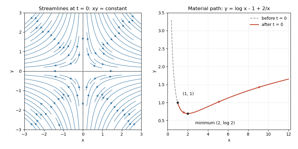
The divergence is ${\partial }_x{u}_x+{\partial }_y{u}_y=1-1=0$, while the scalar vorticity is ${\partial }_x{u}_y-{\partial }_y{u}_x=0$. The flow is therefore incompressible flow and irrotational flow. Integrating the streamfunction equations givesThe time dependence must be retained: no time-independent function $\psi (x,y)$ represents this unsteady field for every $t$. At $t=0$ the streamlines are $xy=\mathrm{constant}$, with the coordinate axes as separatrices. Their arrows point towards increasing $|x|$ and decreasing $|y|$, as shown below.

A pathline solves the material ODEs, givingFor $x_0\ne 0$, elimination of time yieldsIf $x_0=0$, the pathline stays on the $y$ axis and the parametric expression remains valid; it cannot in general be written as a single-valued $y=f(x)$ along that vertical trajectory. For $x_0=y_0=1$, the path is $y=\log x-1+2/x$: it initially descends, reaches its minimum $(2,\log 2)$, then rises. Unlike a frozen streamline, it records the time-varying flow.

Use the upper-half-plane model of the hyperbolic plane, whose geodesics are vertical lines and semicircles perpendicular to the real boundary. Hyperbolic and Euclidean angles agree. An isometry takes one of the ultraparallel hyperbolic lines to the imaginary axis. The other then has two finite endpoints on the same side; reflecting if necessary, write them as $0<a<b$. Its Euclidean centre and radius are $c=(a+b)/2$ and $r=(b-a)/2$.

A geodesic perpendicular to the imaginary axis must be a semicircle centred at zero, of some radius $q$. Two intersecting Euclidean circles meet orthogonally exactly when their squared centre distance equals the sum of their squared radii. Orthogonality to the second line therefore requiresSince $a<\sqrt{ab}<b$, the two semicircles intersect at one point in the upper half-plane. This constructs the common perpendicular of ultraparallel hyperbolic lines and proves uniqueness, because its radius is forced.

For the three-line continuation, the three common perpendiculars can be pairwise disjoint, but need not be. Explicit configurations of three ultraparallel lines make both claims transparent. For the positive example, take the three semicircles of radius $1/2$ centred at $-5/2,0,5/2$. Their endpoint intervals are disjoint. Their common perpendiculars are the semicircles with centres $-5/4,5/4,0$ and radii $\sqrt{21}/4,\sqrt{21}/4,\sqrt{6}$, respectively. The two smaller semicircles are disjoint because $2(\sqrt{21}/4)<5/2$; each is nested inside the largest because $5/4+\sqrt{21}/4<\sqrt{6}$. Hence their full geodesics are disjoint. For the negative example, take three concentric semicircles of radii $1,2,3$. They are pairwise ultraparallel, but every common perpendicular is the imaginary axis, so the perpendiculars coincide.

The adjugate matrix is the transpose of the cofactor matrix: $\mathrm{adj}(A{)}_{ij}=(-1{)}^{i+j}\det A_{\hat{j},\hat{i}}$. Cofactor expansion gives the adjugate identityFor an invertible matrix this yields $A^{-1}=\mathrm{adj}(A)/\det A$. Integer entries of $A$ imply integer cofactors, so $\det A=\pm 1$ makes its inverse integral. Conversely, if $A$ and $A^{-1}$ both have integer entries, their determinants are integers and $(\det A)(\det A^{-1})=1$. The only integer units are $\pm 1$. Hence an invertible integer matrix has an integer inverse exactly when it is a unimodular matrix, with determinant $\pm 1$. Invertibility is implicit whenever $A^{-1}$ is used.

Let $H=X(X^{T}X{)}^{-1}{X}^T$ be the orthogonal projection onto the design column space. Linear transformations of the Gaussian errors giveThe residual distribution is a singular multivariate normal supported on the orthogonal complement of that column space. Their cross-covariance is ${\sigma }^2(X^{T}X{)}^{-1}{X}^T(I-H)=0$. Joint normality even makes the two vectors independent.

Order the observations as $11,12,21,22$. The two normal linear models have design matricesRemoving each row mean leaves the information for the common slope equal to the sum of within-row squared fertilizer deviations. These sums are $1$ and $4$, respectively. ThereforeThe second design estimates the slope four times as precisely in variance terms.

The observed data in the second design are fitted exactly by $\hat{\theta }=(100,300,100{)}^T$. With $a=(2,2,0{)}^T$, the no-fertilizer total forecast isThe future four independent errors contribute variance $4{\sigma }^2$. Parameter-estimation uncertainty contributes ${\sigma }^2{a}^T(X_{II}^T{X}_{II}{)}^{-1}a=13{\sigma }^2$, so the prediction-error variance is $17{\sigma }^2$, not merely the variance of the estimated mean. Normally, with $s^2=\Vert \widehat{ϵ}{\Vert }^2/(4-3)$, the prediction interval in a normal linear model isHere the printed data have zero residual and hence $s=0$. The formal plug-in interval collapses to $[800,800]$, exhibiting zero-residual degeneracy of regression prediction. Under the stated model with unknown positive variance, this exact fit is a probability-zero sample and the Studentized statistic is undefined at it; the collapsed expression is not evidence that future yield is certain. No positive-width numerical 95% interval can be obtained from these exact data by the usual residual-variance method without extra variance information or an explicit observation-rounding model.

For a full-column-rank matrix, a thin QR decomposition has $A=Q_{1}R$, where $Q_1^T{Q}_1=I_n$ and $R$ is nonsingular upper triangular. Extend $Q_1$ to an orthogonal matrix $Q=(Q_1,Q_2)$. Orthogonality givesThus the unique least-squares solution satisfies $R{x}^{\ast }=Q_1^{T}b$, with residual norm $\Vert Q_2^{T}b\Vert$. In a rank-deficient problem $R$ is singular and uniqueness needs separate treatment.

A Givens rotation is the identity except for the rows/columns $p,q$, whose block is $\left(\begin{array}{cc}c& s\\ -s& c\end{array}\right)$ with $c^2+s^2=1$. Its transpose times itself has that block equal to the identity, so it is orthogonal. Choose $c=4/5,s=3/5$ in rows two and three. ThenBack substitution in the first three rows givesThe fourth row of the rotated residual is the unavoidable value $-2$, while the other three rows vanish. Thus this rotation also directly exhibits the least-squares optimality.