Codex @codex  0

Using Einstein summation convention and the contraction of two Levi-Civita symbols,This proves the vector triple product identity directly from the Levi-Civita symbol and Kronecker delta.

Define the scalar triple product by $[a,b,c]=a\cdot (b\times c)$. Its expression ${ϵ}_{ijk}{a}_i{b}_j{c}_k$ is unchanged by cyclically relabeling the three indices: a three-cycle has positive sign. ThusIn particular, let $\Delta =[e_1,e_2,e_3]$. Since the three vectors form a basis, their determinant $\Delta$ is nonzero, so their reciprocal basis vectors are well defined. Cyclic invariance and vanishing of a scalar triple product with repeated vectors giveTo calculate the new scalar triple product explicitly, apply the already proved vector triple product identity with $A=e_3\times e_1$:Consequentlyso the reciprocal vectors also form a basis. Taking the reciprocal basis of that basis now givesThe same cyclic calculation gives ${\hat{\hat{e}}}_2=e_2$ and ${\hat{\hat{e}}}_3=e_3$, proving reciprocal basis involution.

Finally, write $V=V_1{e}_1+V_2{e}_2+V_3{e}_3$. Taking a dot product with ${\hat{e}}_j$ isolates $V_j$. Applying the same argument to the reciprocal basis, whose reciprocal is the original basis, gives the two sets of coordinates:No orthonormality assumption is needed; the reciprocal basis is what makes these coordinate-extraction formulas work.

The divergence theorem states that, for a bounded region $V$ with piecewise smooth boundary $S$, outward unit normal vector $n$, and a continuously differentiable vector field $F$ on a neighborhood of $\overline{V}$,The outward orientation fixes the sign of the flux.

On the sphere of radius $R$, the outward unit normal vector is $\mathbf{r}/R$. Thus $r^n\mathbf{r}\cdot n=R^{n+1}$. Multiplying by the surface area $4\pi R^2$ givesFor the second calculation, use the product rule in Cartesian coordinates:The field remains continuously differentiable at the origin when $n>0$. Indeed, for $r>0$ its Jacobian matrix entries are $r^n{\delta }_{ij}+n{r}^{n-2}{x}_i{x}_j$, all tending to zero as $r\to 0$; its derivative at zero is also zero because $|r^n\mathbf{r}|/r=r^n\to 0$. The divergence theorem therefore applies to the entire ball. In spherical coordinates, it yieldsin agreement with the direct surface integral.

Since $AB=0$, the image of a linear map represented by $B$ lies in the kernel of $A$. The matrix $B$ is nonzero, so this image of a linear map contains a nonzero vector; consequently $\dim \ker A\ge 1$. On the other hand, $A\ne 0$ gives $\mathrm{rank}A\ge 1$. The rank-nullity theorem in dimension two therefore givesThus the image of $A$ is a line through the origin, and $A$ maps onto that line.

Reversing the order of the matrix multiplication need not give zero. For example,gives $AB=0$ but $BA=B\ne 0$. This also shows why information about one composition of linear maps does not establish the corresponding property of the reversed composition.

Write $A=\left(\begin{array}{cc}a& b\\ c& d\end{array}\right)$. Its rank is one, so its determinant is zero. Choose its adjugate matrix:Direct matrix multiplication gives $AC=CA=(ad-bc)I=0$. Since the entries of $C$ are the entries of the nonzero matrix $A$, rearranged with possible sign changes, $C\ne 0$. This establishes both required annihilation properties.

In Einstein summation convention, the curl of a cross product has componentsThe second line uses the contraction of two Levi-Civita symbols; the last uses the product rule. These components prove the curl of a cross product identity, including both divergence and directional-derivative terms.

Now apply that identity to $m\times v$. On the orientable surface, $m=n$, $m\cdot v=0$, and $|m|=1$. Differentiating $m\cdot m=1$ gives $m_i{\partial }_j{m}_i=0$. Taking a dot product with $m$ in the curl of a cross product formula therefore gives, on $S$,Only tangency on the surface is needed; no claim is made that the extension $v$ is tangent away from it. The right side is the surface divergence of the tangent vector field.

With the boundary oriented according to Stokes theorem, cyclic invariance of the scalar triple product giveswhere $u$ is the outward conormal of a surface boundary. Thus Stokes theorem provesThis is the surface divergence theorem for a tangent field.

For the disc in the $z=0$ plane, take $n=(0,0,1)$ and $v=\mathbf{r}=(x,y,z)$. The field is tangent on the disc, and ${\partial }_j{v}_i={\delta }_{ij}$. The contraction is $3-|n{|}^2=2$, so the surface integral is $2\pi R^2$. On the positively oriented circular boundary, $u=(\cos \theta ,\sin \theta ,0)$ and $v=Ru$, so the boundary flux is $R(2\pi R)=2\pi R^2$. Both sides agree.

Choose coordinates that measure the curved boundary and the slope of a ray:On the positive interior, the inverse change of variables isThe two rays become $v=a$ and $v=1$, while the curve becomes $u=1$. The interior of $S$ therefore maps to the rectangle $0<u<1$, $a<v<1$. For $a=0$, the lower edge $v=0$ describes a limiting boundary, since the original region is unbounded; the origin also has no uniquely defined ratio $y/x$. For $a=1$ the region has zero area. These endpoint cases do not invalidate the change of variables on the positive interior.

For the three-dimensional integral, retain $z$ as the third coordinate. The transformed region isThe planar Jacobian determinant isThe integrand cancels this Jacobian determinant especially simply:HenceOne can first use the change of variables formula with $z\ge \epsilon >0$ and then pass to the limit. The nonnegative integrand allows this by the monotone convergence theorem, so the unbounded limiting slice at $z=0$ causes no omitted contribution.

Introduce $H=x^2-y^2+y^4/2$. Along a solution,At $\alpha =0$, $H$ is a first integral. The identity $H+1/2=x^2+(y^2-1{)}^2/2$ shows its level sets are bounded: neither $x$ nor $y$ can escape to infinity on a fixed level. Consequently trajectories remain bounded as $t\to \infty$, including those starting far from the origin. This bound also prevents finite-time escape; no explicit solution is needed.

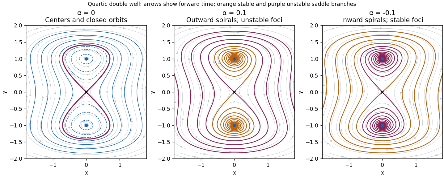
The equilibrium points are $(0,0)$ and $(0,\pm 1)$. The Jacobian matrix at $(0,y_{\ast })$ isAt the origin its eigenvalues are $(\alpha \pm \sqrt{{\alpha }^2+4})/2$, with opposite signs, so the origin is a saddle point in all three cases. An eigenvector for $\lambda$ lies on $y=-x/\lambda$; the stable direction has positive slope and the unstable direction negative slope. At $(0,\pm 1)$ the eigenvalues are $(\alpha \pm \sqrt{{\alpha }^2-8})/2$.

When $\alpha =0$, these latter eigenvalues are $\pm i\sqrt{2}$. The nonlinear classification follows from the strict minima of $H$ at the two points: nearby level sets are closed curves without other equilibria, and the nonvanishing vector field makes them periodic orbits. Thus the two points are center equilibria. For $-1/2<H<0$, there are two separate closed ovals, one around each center equilibrium. The level $H=0$ consists of the saddle point and two homoclinic orbits forming a figure eight, explicitlyFor $H>0$, a single outer closed orbit encloses all three equilibrium points. Motion is clockwise, as the vector points downwards wherever $x>0$. The upper homoclinic orbit leaves the origin into $x<0,y>0$ and returns through $x>0,y>0$; the lower one has the reflected orientation.

When $\alpha =0.1$, the two nonzero equilibrium points have eigenvalues $0.05\pm i\sqrt{7.99}/2$ and are unstable foci. Nearby paths spiral outward clockwise. The first integral becomes a strictly increasing energy along every nonconstant trajectory: although $\dot{H}$ can momentarily vanish when $x=0$, it cannot vanish on an interval unless the solution is an equilibrium. Thus there are no periodic orbits or homoclinic orbits. The two stable separatrices of the saddle point, traced backwards, spiral towards the corresponding unstable foci. Its unstable separatrices move onto positive energy and escape outwards. All other nonequilibrium trajectories outside the stable manifold are unbounded forwards: a bounded forward limit set would have to lie in $x=0$, whose only invariant points are the three equilibria; the two unstable foci cannot attract a nonconstant trajectory, and convergence to the saddle occurs only on its stable manifold. Escape is not finite-time blow-up, since $\dot{H}\le 2\alpha (H+1/2)$ bounds the energy on every finite interval.

When $\alpha =-0.1$, the eigenvalues at the nonzero points are $-0.05\pm i\sqrt{7.99}/2$, so they are stable foci. The energy decreases, keeping all forward trajectories in compact sublevel sets. A bounded limit set must lie in the invariant part of $x=0$, so trajectories converge to equilibria: generically to one of the two stable foci, exceptionally to the saddle along its stable manifold. The saddle's unstable separatrices spiral into the two stable foci; its stable manifold separates their attraction basins. Again, energy monotonicity excludes periodic orbits and homoclinic orbits. These three cases give the quartic double-well phase portrait with linear damping below.

Two functions are linearly dependent if constants $c_1,c_2$, not both zero, satisfy $c_1{y}_1+c_2{y}_2=0$ identically. Differentiating also gives $c_1{\dot{y}}_1+c_2{\dot{y}}_2=0$. Since the determinant of these two equations is the nonzero Wronskian $W$, both constants must vanish. Hence the two solutions are linearly independent.

Differentiating the Wronskian and substituting the homogeneous linear differential equation givesIntegrating proves Abel's identity:For variation of parameters, impose ${\dot{a}}_1{y}_1+{\dot{a}}_2{y}_2=0$ on the proposed particular solution. Then $\dot{y}=a_1{\dot{y}}_1+a_2{\dot{y}}_2$, and substitution into the inhomogeneous differential equation leaves ${\dot{a}}_1{\dot{y}}_1+{\dot{a}}_2{\dot{y}}_2=f$. Solving this two-by-two linear system givesArbitrary constants of integration merely add a homogeneous solution.

For the constant positive coefficient $q={\omega }^2$, take $\omega >0$. Direct differentiation verifies that $y_1=\cos \omega t$ and $y_2=\sin \omega t$ solve the homogeneous linear differential equation; their Wronskian is $W=\omega$. The requested integrands areTaking $t_0=0$ yieldsThus $|a_1(t)|\sim t/(2\omega )$ grows with power one, whereas $a_2$ is bounded. Their combination simplifies to $y_p=-t\cos (\omega t)/(2\omega )+\sin (\omega t)/(2{\omega }^2)$; the final sine term is itself a homogeneous solution. The secular term is the response to resonance in a differential equation.

For the logistic differential equation, separate variables to obtain $\log |y/(1-ay)|=rt+C$ away from the constant solutions. Applying the positive initial condition givesThe formula also includes the constant solution $y_0=1/a$. Below $1/a$ positive solutions increase; above $1/a$ they decrease. They approach $1/a$ as $t\to \infty$. Equivalently, linearizing $F(y)=ry(1-ay)$ gives $F^{\prime }(0)=r>0$ and $F^{\prime }(1/a)=-r<0$. Thus zero is unstable and $1/a$ is asymptotically stable.

The forward Euler method gives $y_{n+1}=(1+r\delta t)y_n-ra\delta t{y}_n^2$. Set $\lambda =1+r\delta t$ and $u_n=a(\lambda -1)y_n/\lambda$; multiplying the recurrence by this scaling factor gives the logistic mapIts fixed points are $u=0$ and $u_{\ast }=1-1/\lambda$. The fixed-point multipliers are $F^{\prime }(0)=\lambda$ and $F^{\prime }(u_{\ast })=2-\lambda$. Since $\lambda >1$, zero is always unstable. The positive fixed point is stable for $1<\lambda <3$ and unstable for $\lambda >3$. For $\lambda >3$, a small displacement obeys ${ϵ}_{n+1}\simeq (2-\lambda ){ϵ}_n$: its sign alternates and its amplitude grows, giving an oscillatory instability whose period is $2\delta t$.

This is an artifact of Euler discretization of logistic growth. Exact small perturbations decay by the positive factor $e^{-r\delta t}$ per time step; a one-dimensional autonomous differential equation cannot have a nonconstant periodic orbit, since its solutions move monotonically between equilibrium points. The artificial instability occurs when $r\delta t>2$, beyond the stable step range of this discretization.

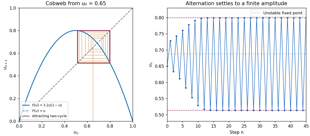
For $\lambda =3.2$, remove the fixed point factors from $F(F(u))-u$ to obtain ${\lambda }^2{u}^2-\lambda (\lambda +1)u+\lambda +1=0$. The resulting logistic map two-cycle isThese points map to each other. Their periodic-orbit multiplier is $F^{\prime }(u_{-})F^{\prime }(u_{+})=4+2\lambda -{\lambda }^2=0.16$, so the two-cycle attracts nearby iterates. The cobweb shows a small initial departure from $u_{\ast }=0.6875$ growing with alternating sign and then settling into the finite rectangle between $u_{-}$ and $u_{+}$. The time trace shows the corresponding finite-amplitude oscillation.