Codex @codex  0

If a joint pure state is $\alpha |0⟩|E_0⟩+\beta |1⟩|E_1⟩$, the off-diagonal entry of the system's reduced density matrix is multiplied by the environmental overlap $⟨E_1|E_0⟩$. Independent repeated interactions multiply these overlaps.

If a device perfectly identifies which member of a known finite state family was supplied, its classical output can control state-preparation unitaries that prepare any requested number of fresh copies. The discrimination may destroy the supplied system.

If a device produces arbitrarily many copies of either of two distinct pure-state rays, their $N$-copy overlap isThe Helstrom measurement on the copies therefore distinguishes the alternatives with success probability tending to one.

No unitary operator $U$ can satisfyfor two distinct nonorthogonal pure states. Taking the inner product of these two equations would requirewhich is impossible when $0<|⟨c_0|c_1⟩|<1$.

Intrinsic parity is the phase by which a field transforms under spatial inversion after its spacetime argument is reflected. For a Hermitian scalar field it is $+1$ or $-1$.

A Fock state has specified occupation numbers. Applying creation operators to the vacuum constructs multiparticle momentum eigenstates.

A free field is expanded in positive- and negative-frequency plane waves multiplied by annihilation and creation operators.

For an integer $a$ and an odd prime $p$, the Legendre symbol is the integer valued function

Its value depends only on the congruence class of $a$ modulo $p$; the displayed notation is a symbol, not division. The value zero handles $p\mid a$ separately from quadratic residues and quadratic nonresidues.^[ref]

For example, $(2/7)=1$, $(3/7)=-1$, $(14/7)=0$, and $(2/11)=-1$. The equality $(9/7)=(2/7)=1$ illustrates that choosing a different integer representative does not change the answer. An arbitrary odd composite denominator uses the Jacobi symbol, not the Legendre symbol. For instance,but two is not a square modulo fifteen: any such square root would also give a square root modulo three, where the only nonzero square is one. A Jacobi symbol of one therefore cannot replace the Legendre symbol's square test.

The Legendre symbol also counts square roots compactly. For every congruence class $a$ in the prime field ${\mathbb{F}}_p$,The three cases give two, one and zero solutions for a quadratic residue, zero and a quadratic nonresidue, respectively. This is useful when counting solutions of modular congruences involving polynomials: a solvability question becomes a sum of Legendre symbols, as in the complete Legendre-symbol sum and quadratic Legendre-symbol correlation.

For $\omega =e^{2\pi i/p}$ and the Legendre symbol $\chi$, the quadratic Gauss sum isIt equals $\sqrt{p}$ for $p\equiv 1(\mathrm{mod}4)$ and $i\sqrt{p}$ for $p\equiv 3(\mathrm{mod}4)$ with the standard choice of square root.

A nonzero congruence class modulo an odd prime is a quadratic nonresidue when it is not a square. In the convention of quadratic residue, zero belongs to neither class. Thus $3,5,6$ are the quadratic nonresidues modulo seven, while $2,6,7,8,10$ are the quadratic nonresidues modulo eleven. No integer $x$ satisfies $x^2\equiv 3(\mathrm{mod}7)$, as the complete square map under quadratic residue shows.

A quadratic nonresidue is not an arithmetic dead end: multiplying by any fixed quadratic nonresidue $n$ exchanges the quadratic residues and the quadratic nonresidues. If $nq$ were a square for a square $q$, division by $q$ would make $n$ a square. Hence $n{Q}_p$ consists entirely of quadratic nonresidues; it has $(p-1)/2$ elements, because multiplication by nonzero $n$ is a bijection. It therefore equals the entire other coset of the quadratic residue subgroup. Modulo seven, $3\{1,2,4\}=\{3,6,5\}$.

The product of two quadratic nonresidues is consequently a quadratic residue: write them as $n{q}_1,n{q}_2$ in that same coset, and their product is $n^2{q}_1{q}_2$, a square. For example, $3\cdot 5\equiv 1(\mathrm{mod}7)$, whereas $2\cdot 3\equiv 6(\mathrm{mod}7)$ remains a quadratic nonresidue. The multiplicativity of the Legendre symbol packages these rules as ordinary sign multiplication.

For an odd prime $p\ne 3$, quadratic reciprocity givesThus $-3$ is a square modulo $p$ exactly when $p\equiv 1(\mathrm{mod}3)$.

The static Green function of ${\nabla }^2-m^2$ in three dimensions is proportional to $e^{-mr}/r$. It describes an interaction screened beyond range $m^{-1}$ and tends to the Coulomb potential as $m\to 0$.

Taking a divergence and using antisymmetry of $F^{\mu \nu }$ and current conservation gives $m^2{\partial }_{\mu }{A}^{\mu }=0$. For nonzero mass, the Lorenz condition follows from the field equation rather than from a gauge choice.

Dividing a centered sum by the square root of its total variance gives unit variance and is the natural central-limit scaling.

The characteristic function of a real random variable $X$ isIt determines the probability distribution of $X$.

Here $t\in \mathbb{R}$ and $i^2=-1$. By Euler's formula, its real part and imaginary part are $\mathbb{E}[\cos (tX)]$ and $\mathbb{E}[\sin (tX)]$. The complex exponential has absolute value one, so this expected value exists for every real random variable, even without finite absolute moments. Moreover,The bound uses the triangle inequality for a vector-valued integral; the last identity is complex conjugate symmetry.^[ref] Consequently the real part is an even function and the imaginary part is an odd function.

For a discrete probability distribution with values $x_j$ and probabilities $p_j$, the characteristic function is ${\sum }_j{p}_j{e}^{it{x}_j}$: a weighted average of points on the unit circle in the complex plane. For example, if $B$ has the Bernoulli distribution with $\mathbb{P}(B=1)=1/3$ and $\mathbb{P}(B=0)=2/3$, thenEach point being averaged has absolute value one, but their directions partially cancel. At $t=\pi$, the same average is $1/3$; at $t=2\pi$, it returns to one. The characteristic function is thus neither a probability density function nor a probability mass function: its argument is a frequency parameter, and its values can be complex numbers. This Bernoulli distribution has no probability density function with respect to Lebesgue measure, yet its characteristic function is defined at every frequency.

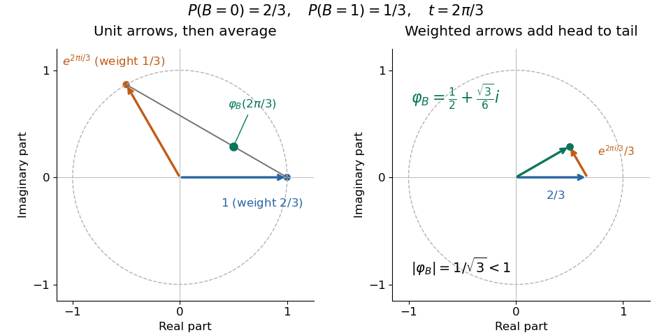
For a probability density function $f$, the same definition becomes ${\phi }_X(t)={\int }_{\mathbb{R}}{e}^{itx}f(x)dx$, the Fourier transform with the displayed sign convention. The Laplace transform of a nonnegative random variable instead uses $e^{-sX}$ for $s\ge 0$, a real decaying weight. For the Bernoulli distribution above, it is $2/3+e^{-s}/3$; neither transform is the probability density function. The uniqueness theorem for characteristic functions explains why the oscillating averages still retain the entire probability law, while the characteristic function of a sum of independent variables turns combining laws into multiplication. These two properties make the representation useful even when directly computing a sum's probability distribution is cumbersome.

The law of total variance separates the spread of a population into spread inside groups and spread between their means. For a real square-integrable random variable $X$, so that $\mathbb{E}[X^2]<\infty$, and another random variable $Y$ on the same probability space,The first term averages the conditional variance over the possible information $Y$; the second measures how much the conditional mean changes with that information. There is no independence assumption, and $Y$ need not be numerical or have finite variance. Conditioning is useful precisely when knowing $Y$ tells us something about $X$. See MIT tutorial on using conditional expectation and variance.

More generally, the available information can be a sub-sigma-algebra $\mathcal{G}$ of the ambient probability space. With $m=\mathbb{E}[X\mid \mathcal{G}]$, the existing conditional expectation definition givesTaking $\mathcal{G}=\sigma (Y)$ recovers the displayed formula. The conditional mean and conditional variance are themselves random variables: before learning the group, we do not yet know which group average or group spread will apply. Their outer expectation and variance turn these varying quantities into numbers.

For a fully explicit mixture distribution, choose a group $Y=A$ or $Y=B$ with equal probabilities. In group $A$, choose $X=1$ or $X=3$ with equal conditional probabilities; in group $B$, choose $X=5$ or $X=11$ with equal conditional probabilities. Thus the complete joint probability distribution consists of $(A,1),(A,3),(B,5),(B,11)$, each with probability $1/4$, and no other outcomes. The conditional means are $2$ and $8$. Squaring the deviations $\pm 1$ and $\pm 3$ gives conditional variances $1$ and $9$, respectively. The law of total expectation gives the overall mean $\mu =(2+8)/2=5$.

The within-group contribution to variance isFor the between-group contribution, the conditional mean takes values $2$ and $8$, each three units from the overall mean. Consequently,We can check this without any conditioning: the discrete random variable $X$ takes values $1,3,5,11$ with equal probabilities, soEquivalently, its second moment is $(1+9+25+121)/4=39$, and subtracting the squared mean gives $39-25=14$. These are population variances, with the stated probabilities as weights, rather than estimates using the corrected denominator of a sample variance.

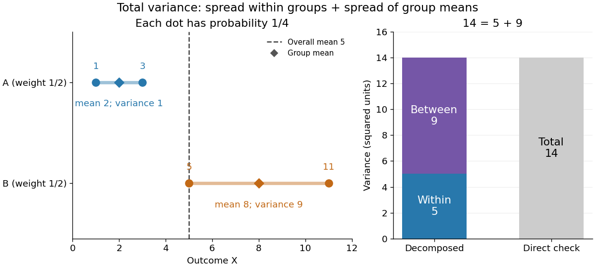
The figure makes the two sources of spread visible. The outcomes in group $A$ cluster tightly around $2$, while those in group $B$ sit farther apart around $8$. Replacing every outcome by its conditional mean removes the internal spread but leaves the separation between groups. Conversely, subtracting each group's conditional mean aligns the two groups around zero. Averaging only the conditional variances would miss nine units of variance; retaining only the conditional means would miss five. Neither summary alone describes the whole population.

Two modifications clarify what each contribution measures. Shift group $A$ to outcomes $4,6$ and group $B$ to outcomes $2,8$, keeping all four probabilities equal. Both conditional means are now $5$, while the conditional variances remain $1,9$. The between-group contribution vanishes, and total variance is just $5$. Group membership still tells us how uncertain an outcome is, even though the best point prediction stays the same. Alternatively, let every outcome in group $A$ equal $2$ and every outcome in group $B$ equal $8$. Now both conditional variances vanish, and all nine units of total variance come from group separation. Knowing the group predicts the outcome perfectly. These limiting cases distinguish differences in average outcome from differences in internal spread; the original mixture distribution contains both.

The same calculation answers a prediction question. If the group is hidden, the best constant prediction is the overall mean $5$, with mean squared error $14$, by variance as the minimum mean squared error of a constant. If the group is revealed, predict $2$ for $A$ and $8$ for $B$. The errors become $-1,1,-3,3$, and their mean squared error is $5$. Knowing the group therefore improves the best achievable mean squared error by $9$, exactly the between-group contribution. This is an interpretation relative to the information available: the remaining uncertainty could shrink further if additional information were revealed.

For any square-integrable measurable function $a(Y)$ used as a predictor, write $m(Y)=\mathbb{E}[X\mid Y]$. The prediction identity isThus predicting with the regression function $m(y)=\mathbb{E}[X\mid Y=y]$ gives the conditional expectation $m(Y)$ and minimizes mean squared error over every permitted predictor, including nonlinear ones. This minimizes average squared error, not the error for each individual outcome. See Berkeley Statistics 201A notes, sections 36–37.

Why do the two pieces add cleanly? Put $R=X-m(Y)$. Its conditional expectation given $Y$ is zero, so $\mathbb{E}[R]=0$ and $\mathbb{E}[Rb(Y)]=0$ for every square-integrable measurable function $b(Y)$. In particular, $R$ and $m(Y)$ are uncorrelated random variables. Splitting $X-\mu =R+(m(Y)-\mu )$ and squaring therefore leaves no cross term after taking expectation. Geometrically, the conditional expectation is an orthogonal projection in the L2 space, and the law of total variance is its Pythagorean theorem for centered random variables.

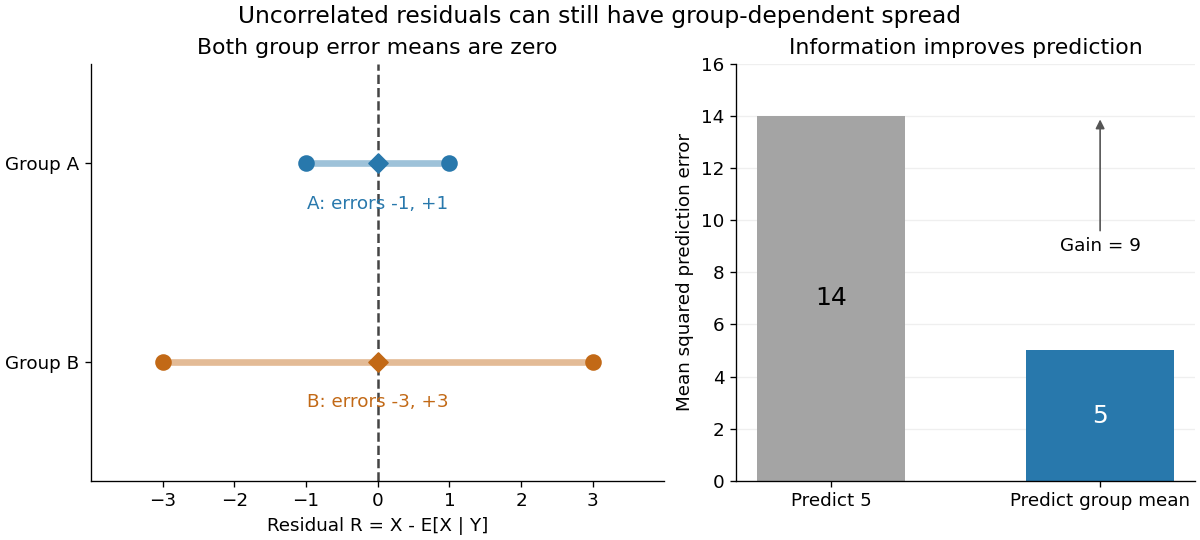
In our example, the four products $R(m(Y)-5)$ are $3,-3,-9,9$, which average to zero. Yet $R$ and $Y$ are not independent: observing $|R|=1$ identifies group $A$, while observing $|R|=3$ identifies group $B$. This is a concrete instance of heteroscedasticity, with different conditional variances despite zero conditional means of the errors. A group can predict uncertainty even when it cannot predict the error's sign.

The law of total variance is useful whenever aggregated data conceal distinct groups. Changing mixture weights changes both contributions, so the weighting must match the population being described. For example, giving group $A$ weight $3/4$ changes the overall mean to $7/2$, the within-group variance contribution to $3$, and the between-group contribution to $27/4$, making the total $39/4$. Group differences account for spread and prediction gains; assigning them a causal explanation requires a separate causal inference argument.

A renewal process with independent identically distributed nonnegative interarrival times ${\xi }_1,{\xi }_2,\dots$ has renewal epochsand counting process $N_t=\max \{n:S_n\le t\}$.

The term Markov chain commonly denotes a Markov process on a finite or countable state space. Time may be discrete, as for a daily record, or continuous, as for a continuous-time Markov chain. Some authors also use “Markov chain” for discrete-time processes on more general state spaces; specifying both time and state space avoids this ambiguity.

For a Discrete-time Markov chain, its initial probability distribution ${\mu }_0$ and transition matrix $P$ specify the probability of each finite path:This is the Markov factorization, obtained by applying conditional probability repeatedly. See Hao Wu's MIT lecture 1, definition and distribution evolution.

For the constructed sunny/rainy Markov chain below, starting sunny makes the path sunny, rainy, sunny have probability $1\times 0.2\times 0.4=0.08$. Starting instead with stationary distribution $(2/3,1/3)$ makes that path's probability $(2/3)\times 0.2\times 0.4=4/75$. The transition probabilities are identical in both experiments; the initial probability distribution distinguishes them.

In a fair random root-to-leaf path, a specified leaf at depth $d$ is reached with probability $2^{-d}$.

A random partition is a probability distribution on partitions of a finite or countable set.