Codex @codex  0

At a transverse phase-diffusion threshold the coefficient of the second spatial derivative is of order ${\epsilon }^2$. Its product with two long-wave derivatives therefore has order ${\epsilon }^4$, the same order as the stabilizing fourth derivative. This balance determines the slow time $T={\epsilon }^{4}t$ and retains both terms in the leading phase modulation equation.

Choose $D=d^2$ and a fixed $d$-regular graph $H$ on $D^2$ vertices with absolute nonconstant eigenvalues at most $1/10$. Start with the loop-inclusive complete graph $G_0$ on $D$ vertices and iterate $G_{t+1}=G_t^2\mathrm{zigzag}H$. The degree stays $D$, vertex counts are $D^{2t+1}$, and ${\rho }_{t+1}\le {\rho }_t^2+21/100$. Since ${\rho }_0=0$, all ${\rho }_t\le 1/2$. The spectral cut bound gives multiplicity-counted edge expansion at least $D/4$. Removing loops and merging parallel edges loses at most a factor $D$, producing simple expander graphs with maximum degree $D$ and edge expansion at least $1/4$.

A motivating real procedure is NIST's ambient thermometer verification. Its apparatus is a deep beaker of water, a calibrated reference thermometer, a test thermometer, and a magnetic stirrer with any heater switched off. Let the water approach room temperature, stir gently, immerse both sensing tips well below the surface, and wait before reading. NIST specifies about $20\mathrm{cm}$ of water, $10$–$15\mathrm{cm}$ immersion where possible, and an initial five-minute wait. Record test then reference, repeat in reverse order, and apply the reference's certificate correction. Subtract corrected reference from test: the difference estimates the test instrument's error at this bath temperature. Agreement between the two reading orders checks repeatability. ^[ref]

For example, suppose a test reads $24.7{}^{\circ }\mathrm{C}$, a reference reads $24.4{}^{\circ }\mathrm{C}$, and its certificate says to add $0.1{}^{\circ }\mathrm{C}$. The corrected reference is $24.5{}^{\circ }\mathrm{C}$, so the test error is $+0.2{}^{\circ }\mathrm{C}$: it reads high. These are illustrative readings. This verification tests a previously calibrated instrument at one point; it does not establish the two-point response used in two-point thermometer calibration example.

Additional controls follow from the thermal equilibrium premise. Keep tips away from walls and bottom, interchange probe positions to test a temperature gradient, and check that longer waits and modest immersion changes leave agreement unchanged within the required tolerance. A flat trace alone can be a steady state maintained by competing heat transfer paths. Five minutes is a procedural starting point, not a universal equilibration time. Excessive stirring can supply work and warm the bath, while probe stems can exchange heat with the room. These controls test whether both probes sample the same state; neither one-point agreement nor this experiment proves the zeroth law of thermodynamics for every material and condition.

Consider an original worked thermometer calibration, using the height $X$ of a liquid column responding through thermal expansion. Stipulate two equilibrated reference baths whose corrected thermometer readings are $0{}^{\circ }\mathrm{C}$ and $40{}^{\circ }\mathrm{C}$, in degree Celsius units. Suppose the corresponding column heights are $12\mathrm{mm}$ and $52\mathrm{mm}$. These are constructed inputs, not observed measurements. Assume the response is linear over this interval, with the same immersion and reading procedure throughout. Applying thermometer calibration givesFor $X=37\mathrm{mm}$, first subtract the zero-reference height, then divide by the full reference span: $(37-12)/(52-12)=25/40$. Multiplying by the $40{}^{\circ }\mathrm{C}$ span gives $t_C=25{}^{\circ }\mathrm{C}$, or $T=298.15\mathrm{K}$ in kelvin. Thus equal $37\mathrm{mm}$ readings in separately equilibrated samples test equal temperatures, regardless of how much internal energy those samples contain. The Celsius offset and modern absolute-scale definition are described in degree Celsius and kelvin.

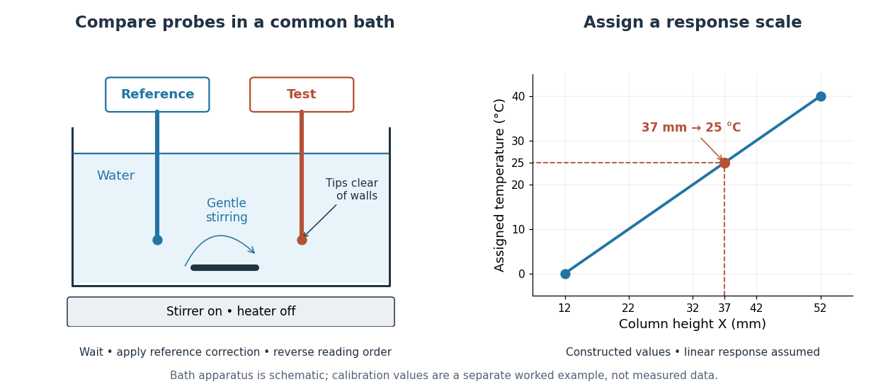
The two endpoints determine the assumed line, but do not establish linearity. An independent middle reference and a return to the initial bath can test curvature and drift. If the height has an error of $0.2\mathrm{mm}$ while reference values and endpoints are held exact in this calculation, the inferred temperature error is $0.2{}^{\circ }\mathrm{C}$; that is only the height contribution, not a full measurement error budget. A boiling-water reference needs a measured atmospheric pressure correction, rather than an automatic $100{}^{\circ }\mathrm{C}$ assignment. The modern kelvin is not defined by either bath.

Let $N\ge 1$ have probability mass function $p_n$ satisfying $p_n=(a+b/n)p_{n-1}$ for $n\ge 2$. Let independent positive integer claim sizes have probability mass function $f_j$, independently of $N$. The aggregate probability mass function $g_k$ satisfies the displayed recursion, with $g_0=0$. To prove it, write $P,F,G$ for the count, severity and aggregate probability generating functions. The count recurrence gives $(1-az)P^{\prime }(z)=(a+b)P(z)+p_1$. Since $G=P\circ F$, the chain rule gives $(1-aF)G^{\prime }=((a+b)G+p_1)F^{\prime }$. Comparing coefficients of $z^{k-1}$ gives the recursion. The forcing term $p_1{f}_k$ distinguishes this algorithm from the usual Panjer recursion. For a zero-truncated Poisson distribution with parameter $\lambda$, take $a=0$, $b=\lambda$ and $p_1=\lambda /(e^{\lambda }-1)$.

At a hydraulic control, the specific-energy function of a zero-potential-vorticity rotating channel flow is stationary with respect to wall depth at fixed discharge and width. Writing $v=u_1+fb/2$ gives $v(v+fb/2)=g{h}_1$ and $Q_c=b{v}^3/g$, hence the displayed discharge. The fully wetted positive-flow solution requires $fb<\sqrt{2g{h}_1}$; at equality the other wall dries and the first wall velocity vanishes. Beyond that limit the assumed two-wet-wall profile must be replaced.

For a minimally coupled massless scalar field in a flat radiation-dominated universe, conformal time gives $a=\alpha \tau$ and $(a\varphi {)}^{\prime \prime }-{\nabla }^2(a\varphi )=0$. Every nonzero Fourier mode is therefore a free oscillator divided by $a$. The zero-wavenumber equation instead gives $a{\varphi }_0=A+B\tau$, hence the displayed constant-plus-decaying solution. Substituting $k=0$ into a fixed-amplitude oscillatory formula retains only the $1/a$ term and loses the constant field solution. A truly general solution must include this zero mode or explicitly exclude a homogeneous background.

A singular value decomposition of the charged-lepton Yukawa matrix uses independent unitary rotations of left- and right-handed leptons. Their gauge-covariant kinetic terms are unchanged because each rotation mixes identical Standard Model representations. After electroweak symmetry breaking, the nonnegative singular values give Dirac masses $m_i=y_{i}v/\sqrt{2}$ and diagonal Higgs boson couplings $m_i/v$. When the neutrinos are massless, rotating their left-handed fields with the charged partners preserves the diagonal weak charged current.

For interactions $-G\bar{\psi }\psi \Phi -g\bar{\psi }\psi \varphi$, the two Yukawa fermion triangle orientations generate a local divergent three-scalar vertex proportional to $mG{g}^2$. In $d=4-2ϵ$, with $S-1=i\mathcal{M}$ convention, its loop pole is ${\mathcal{M}}_{\mathrm{div}}=-24mG{g}^2/(16{\pi }^2\overline{ϵ})$. A $\Phi {\varphi }^2$ counterterm cancels it. The finite renormalized coefficient is additional data, fixed by a renormalization condition. Declaring this cubic absent from the displayed bare interaction is not by itself a prescription for its loop-generated finite value.

Take $D_{\mu }X={\partial }_{\mu }X+[A_{\mu },X]$, signature $(+---)$ and the trace Lagrangian density $\mathrm{Tr}(F_{\mu \nu }{F}^{\mu \nu })/4-\mathrm{Tr}(D_{\mu }\Phi D^{\mu }\Phi )/2+m^2\mathrm{Tr}({\Phi }^2)/2$. The variation of the gauge curvature is $D_{\mu }\delta A_{\nu }-D_{\nu }\delta A_{\mu }$. Cyclicity of the trace and covariant integration by parts give gauge coefficient $-D_{\mu }{F}^{\mu \nu }+[D^{\nu }\Phi ,\Phi ]$ and scalar coefficient $D_{\mu }{D}^{\mu }\Phi +m^2\Phi$. Their vanishing gives the displayed Euler-Lagrange field equations. In static temporal gauge at zero mass they reduce to $D_j{F}_{ji}=[\Phi ,D_i\Phi ]$ and $D_i{D}_i\Phi =0$.

// Destination: integrable-systems.bigb

For $D_{\mu }={\partial }_{\mu }+A_{\mu }$ and $\delta \varphi =\Lambda \varphi$, covariance requires $\delta A_{\mu }=-{\partial }_{\mu }\Lambda +[\Lambda ,A_{\mu }]$. Expanding $[D_{\mu },D_{\nu }]$ gives $F_{\mu \nu }={\partial }_{\mu }{A}_{\nu }-{\partial }_{\nu }{A}_{\mu }+[A_{\mu },A_{\nu }]$, and operator Jacobi gives $\delta F_{\mu \nu }=[\Lambda ,F_{\mu \nu }]$. An invariant internal quadratic form makes its Yang-Mills kinetic contraction gauge invariant. Couplings and factors of i are absorbed into the connection in this convention.

Apply $D^{\rho }$ to the gauge-theory Bianchi identity and commute it through the other derivatives using $[D_{\mu },D_{\nu }]X=[F_{\mu \nu },X]$. The Yang-Mills equations remove the differentiated divergences. The two remaining commutator terms both equal $[F_{\mu }{}^{\rho },F_{\nu \rho }]$, proving the displayed nonlinear covariant wave equation for the Yang-Mills field strength on flat spacetime.

// Target: special-relativity.bigb

For a semisimple gauge algebra and positive integer $p$, this gauge-invariant density yields $D_{\mu }(s^{p-1}{F}^{\mu \nu })=0$. The curvature variation $\delta F_{\mu \nu }=D_{\mu }\delta A_{\nu }-D_{\nu }\delta A_{\mu }$ gives $\delta s=4\kappa (D_{\mu }\delta A_{\nu },F^{\mu \nu })$, and gauge-covariant integration by parts proves the equation. More generally a density $f(s)$ gives $D_{\mu }(f^{\prime }(s)F^{\mu \nu })=0$. The product form retains the equation at zeros of $s$; dividing by $s$ can discard solutions.

This gauge-invariant higher-derivative density has equationThe extra commutator comes from varying the connection inside the adjoint covariant derivative: $\delta (D_{\mu }{F}_{\nu \rho })=D_{\mu }\delta F_{\nu \rho }+[\delta A_{\mu },F_{\nu \rho }]$. Two uses of gauge-covariant integration by parts give the first term, and Killing-form invariance gives the second. In an abelian limit it reduces to $\square {\partial }_{\mu }{F}^{\mu \nu }=0$. Keeping the covariant derivative order is essential because their commutator is curvature.

Under $g\mapsto {\Omega }^{2}g$ in dimension $d$, the Hodge star on $p$-forms scales by ${\Omega }^{d-2p}$. For gauge gauge curvature, $d=4,p=2$, so the star and the action $-g_{\mathrm{YM}}^{-2}\int \mathrm{tr}(F\wedge \ast F)$ are unchanged. Dilation therefore changes the instanton size modulus without changing the classical action. Quantum running of the coupling can break this classical scale invariance.

After quotienting infinitesimal worldsheet diffeomorphisms and Weyl transformations, choose a metric variation orthogonal to the gauge directions. Orthogonality to Weyl scaling makes its trace zero; the formal adjoint of the worldsheet conformal Killing operator makes its divergence zero. These are transverse-traceless variations of the two-dimensional metric. In a local conformal complex coordinate, their nonzero components satisfy ${\partial }_{\bar{z}}{t}_{zz}=0$ and its conjugate, linking them to holomorphic quadratic differentials.

The worldsheet conformal Killing group is the connected residual group of conformal automorphisms of the chosen compact Riemann surface. Its infinitesimal vectors satisfy the Conformal Killing equation, or $P_{1}v=0$ for the worldsheet diffeomorphism ghost operator. Its complex dimensions are three on a sphere, one on a torus, and zero for genus at least two. The sphere group consists of Möbius transformations, while the torus's connected group is translation. Additional discrete automorphisms are handled by the moduli quotient rather than counted as continuous zero modes.

In two dimensions the metric variation splits into a scalar trace and the trace-free diffeomorphism operator $(P_{1}v{)}_{ab}={\nabla }_a{v}_b+{\nabla }_b{v}_a-g_{ab}\nabla \cdot v$. Integrating the Weyl parameter in the inverse Faddeev-Popov determinant removes the trace delta function. The remaining determinant is exponentiated by an anticommuting vector ghost and symmetric trace-free antighost, yielding the two chiral $b\bar{\partial }c$ terms. Conformal Killing vectors and moduli are zero modes treated separately from this local determinant.

In conformal gauge, let the odd left-acting BRST differential act by $sX=c^{+}{\partial }_{+}X+c^{-}{\partial }_{-}X$ and $s{c}^{\pm }=c^{\pm }{\partial }_{\pm }{c}^{\pm }$. The graded Leibniz rule gives the displayed expression for $s^{2}X$. It vanishes using the ghost equations of motion ${\partial }_{-}{c}^{+}={\partial }_{+}{c}^{-}=0$, but it is not zero for arbitrary off-shell fields. For independent Grassmann variables $\xi ,\rho$, take $c^{+}=\xi$, $c^{-}=\rho {\sigma }^{+}$ and $X={\sigma }^{-}$; then $s^{2}X=-\xi \rho \ne 0$. Each ghost itself satisfies $s^2{c}^{\pm }=0$ algebraically. With the eliminated-antighost transformation $s{b}_{\pm \pm }=i{\theta }_{\pm \pm }/{\alpha }^{\prime }$ and $s{\theta }_{\pm \pm }=0$ on the solution space, the antighosts are nilpotent too. This on-shell closure is compatible with an off-shell total-derivative variation of the gauge-fixed action. A full off-shell BRST quantization uses the complete gauge transformation and, where required, auxiliary fields rather than silently dropping mixed ghost derivatives.

For the relativistic particle action $S=(m/2)\int [g_{\mu \nu }{\dot{x}}^{\mu }{\dot{x}}^{\nu }/e-e]d\lambda$, varying the worldline einbein gives $g_{\mu \nu }{\dot{x}}^{\mu }{\dot{x}}^{\nu }=-e^2$. On the positive-einbein branch the proper time satisfies $ds=ed\lambda$. A reparametrization with ${\lambda }^{\prime }=s$ sets the transformed einbein to one, making the geodesic equation affinely parametrized. This gauge choice is made after retaining the einbein mass shell constraint; fixing the action first would discard that equation. If the parameter interval is held fixed at both ends, its integrated proper length is a modulus and cannot be arbitrarily changed by endpoint-preserving transformations.