
Past exam of the geophysical fluid dynamics course of the University of Oxford 2025 2 c ii Solution 2026-10-25
Dense water formed in marginal seas spills over sills and descends the continental slope as a marginal-sea overflow. Strong shear flow generates turbulent mixing and entrainment of surrounding, lighter water. The descending current's volume flux grows while its density anomaly is diluted, modifying the depth at which it joins the deep circulation and the temperature and salinity of the exported water. Thus the deep volume flux can substantially exceed the source overflow volume flux; it cannot be inferred from northern surface cooling alone.[ref]
https://www2.whoi.edu/staff/lpratt/wp-content/uploads/sites/120/2019/07/PrattSec2.11_11823.pdf. Anatomy of an overflow, section 2.11: observed downstream entrainment and dilution of the Faroe Bank Channel overflow
Past exam of the geophysical fluid dynamics course of the University of Oxford 2025 2 c i Solution 2026-10-25
Northern high-latitude cooling removes heat from surface water and raises its density. If the surface water becomes denser than the water below, convection mixes it downward and forms dense water that can be exported in the deep southward branch of the Atlantic meridional overturning circulation. This water-mass transformation helps maintain the contrast represented by in 2(a). Freshening can oppose it by reducing density and increasing stable stratification. Local convection and the basin-integrated sinking volume flux are related but are not the same process: export and the return path also depend on the large-scale dynamics.
Past exam of the general relativity II course of the University of Oxford 2021 1 d ii Solution 2026-10-25
In the prescribed synchronous coordinates, the Christoffel symbols satisfyConsequently the four-acceleration of vanishes. For a spatial index , , so the spatial component of the relativistic Euler equation becomesOn a connected coordinate neighbourhood,A nonzero pressure is allowed, but its spatial gradient must vanish if the fluid's four-velocity follows these freely falling coordinate lines. No division by or is needed.
Past exam of the general relativity II course of the University of Oxford 2021 1 d i Solution 2026-10-25
For relativistic dust, , the relativistic Euler equation gives . The nowhere-vanishing density therefore makes the four-acceleration zero: is a timelike geodesic vector field. Let be the differential one-form obtained by the musical isomorphism. Its exterior derivative satisfiesHere is the interior product. By hypersurface orthogonality and the Frobenius theorem, . Taking the interior product and using givesThus . By the Poincaré lemma, locally , and then . Choose spatial coordinate functions on one level set of and extend them constantly along the integral curves of a vector field , using its smooth flow. This constructs . Since ,The metric on the orthogonal complement of a timelike vector is positive-definite, so the synchronous coordinates for irrotational dust haveThis construction is local; crossing geodesics can prevent these synchronous coordinates from covering a larger region.
Past exam of the general relativity II course of the University of Oxford 2017 2 b iii Solution 2026-10-25
The Killing equation impliesHere , so in the regular coordinatesThis vector vanishes at . The Killing vector field is nonzero there, so comparison with the definition of surface gravity yieldsHence this is a degenerate Killing horizon. The argument uses the vanishing gradient of on the horizon; the condition by itself would not force zero surface gravity.
Past exam of the general relativity II course of the University of Oxford 2017 2 b ii Solution 2026-10-25
On the extension in part (i), the hypersurface has nonzero normal covector . Its squared norm isThis vanishes on , which is therefore a null hypersurface. Raising the index givesSince at fixed , the original Killing vector field becomes the smooth nonzero field . The transformed metric tensor is independent of , so remains a Killing vector field, andThus is both tangent and normal to . This is exactly a Killing horizon:The Killing vector field itself does not vanish there; a vanishing squared norm means nullness, not a zero vector.
Past exam of the general relativity II course of the University of Oxford 2017 2 b i Solution 2026-10-25
A nondegenerate Lorentzian metric requires ; take as the radius convention. The original coordinates describe , with a candidate boundary rather than an ordinary point of that chart. The change of coordinate givesSubstituting and cancelling the two terms proportional to producesThe block of this metric tensor has determinant and inverse metricAll coefficients are smooth through , and the block has one negative and one positive eigenvalue. Together with the positive round two-sphere factor this is a regular Lorentzian metric. It extends to a neighborhood with either sign of . The usual polar-coordinate problem at the poles of the two-sphere is removed by separate angular charts. Therefore is only a coordinate singularity of the original chart. This is the degenerate-horizon patch of Bertotti-Robinson spacetime.
Past exam of the general relativity II course of the University of Oxford 2017 2 a iii Solution 2026-10-25
The product rule for the Lie derivative and the Killing equation giveConsequently is a Conformal Killing vector field for the rescaled metric tensor, with smooth conformal Killing factorIt remains an actual Killing vector field precisely when : the conformal factor must be constant along its integral curves of a vector field.
Past exam of the general relativity II course of the University of Oxford 2017 2 a ii Solution 2026-10-25
Put , which is smooth because is nowhere zero. The conformal change of the Levi-Civita connection isThis follows directly by differentiating and using in the Christoffel symbol formula.
Let be a geodesic tangent for , with an affine parameter. Since ,For a null geodesic the second term vanishes. The remaining acceleration is tangent to the same curve and can be removed by changing its parameter. Explicitly set , with . ThenIt vanishes when , orThis affine parameter change under conformal rescaling shows that conformal preservation of null geodesic paths means preservation of unparametrized curves; the original affine parameter usually changes.
For a non-null geodesic, the component of orthogonal to generally survives. A change of parameter can remove only the tangential component of acceleration. As a concrete example use Minkowski spacetime,The curve is a timelike geodesic for , but along itThis acceleration is not parallel to , so the curve is not a geodesic of under any reparametrization. Special non-null curves may still be preserved, for example when is constant; nullness is the general guarantee.
Past exam of the general relativity II course of the University of Oxford 2017 2 a i Solution 2026-10-25
Since the real conformal factor is nowhere zero, at every point. For any tangent vector,The sign is unchanged. With metric signature , negative, zero and positive values therefore describe the same timelike vectors, null vectors and spacelike vectors for both metric tensors. In particular the two null cones coincide.
Choose the same time orientation for the two Lorentzian metrics. A future-directed causal curve or timelike curve for one has the same character for the other. Hence the causal future, causal past and chronological future of every point agree:This is the preservation of causal structure by a smooth, nonvanishing conformal transformation. It does not assert preservation of proper time or of affine parameter lengths.
Past exam of the general relativity II course of the University of Oxford 2015 3 e ii Solution 2026-10-25
Take the expanding flat branch , with . A radial null geodesic in FLRW spacetime satisfies . For the incoming past light cone of the spacetime event , integration giveswith arbitrary angular direction. Equivalently, conformal time gives .
Let the reception time tend to infinity. The largest comoving radial distance from which a signal emitted at time can reach the central comoving observer isThus the cosmological event horizon has constant proper distance in cosmology:An emitted spacetime event is seen at a finite time if and only if . Equality would require , while an event with never reaches the observer. This is a bound on events at their emission time; a fixed comoving observer can have earlier visible events and later invisible ones.
The boundary really is a null hypersurface. For , its normal has components and , soThe finite future integral, and hence this observer event horizon, uses the expanding branch. For the contracting flat solution , the same integral diverges and there is no future observer event horizon of this kind; the static zero-density solution likewise has none.
Past exam of the general relativity II course of the University of Oxford 2015 3 e i Solution 2026-10-25
For the equation of state , the cosmological continuity equation gives . Hence is constant. First take the physically intended positive energy density and defineThe Friedmann equation and the original Friedmann acceleration equation becomeSolve the second equation as . The first equation then requires . Choosing the time origin separately in each solution gives all positive branches:For , there is also the time reverse on , which contracts to a future zero. For , the cosmological bounce joins contraction to expansion at the positive minimum . Retaining at the minimum excludes a spurious permanently static solution that would satisfy the first-order constraint alone.
These are vacuum-energy FLRW solutions: the expanding flat branch, closed slicing of de Sitter spacetime, and open slicing of de Sitter spacetime. To compare them at the same energy density, the figure sets , takes , and aligns the open boundary and closed minimum at . Thus the three plotted functions are , , and , the last only for .
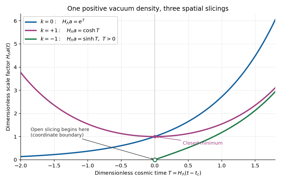
Scale factors for positive vacuum energy: exponential flat expansion, a closed bounce, and open expansion from a finite-time coordinate boundary
. Details. 
Only the expanding branch has a finite past zero. The expanding branch tends to zero only as , and the branch is bounded below. All three describe portions of de Sitter spacetime, with Ricci scalar and Kretschmann scalar . In particular the zero is a boundary of that slicing, not a curvature singularity. The inequality in part (d) does not apply, because .
For zero energy density, the remaining solutions are for , and the expanding or contracting Milne model for ; no positive real solution exists for . If negative energy density is admitted mathematically, write . Only is possible, with for , an open slicing of anti-de Sitter spacetime. These limiting and negative-density cases do not alter the positive-density comparison above.
Past exam of the general relativity II course of the University of Oxford 2015 2 e ii Solution 2026-10-25
With the proper time of the massive test particle, the four-velocity has squared norm :The conserved quantities in part (i) giveMultiplying the normalization by and substituting gives the charged-particle radial equation in Reissner-Nordstrom spacetime:At a radial turning point , the left side is zero, soThe parenthesis on the left is strictly positive. Hence . The factorization in part (b) now yieldsThere is no radial turning point between the horizons. Indeed, for , the right-hand side of the radial equation is strictly positive, independently of the electric charge of the test particle. This is the charged-particle turning-point exclusion in Reissner-Nordstrom spacetime.
The inequalities are necessary, not a claim that a radial turning point exists for every . At a regular horizon crossing a timelike vector cannot be tangent to a null hypersurface, so a massive test particle actually has there. Algebraic equality at would require and does not describe a regular finite-proper time radial turning point on the horizon. In the Schwarzschild spacetime limit , the positive-radius inner alternative disappears.
Past exam of the general relativity II course of the University of Oxford 2015 2 e i Solution Created 2026-10-25 Updated 2026-11-05
On the equatorial path, the Lagrangian per unit mass isBoth and are cyclic coordinates. The Euler-Lagrange equations therefore conserve their canonical momenta:ConsequentlyHere is the total conserved energy in the specified gauge of the electromagnetic four-potential. The paper's is the angular momentum per unit mass; the physical angular momentum is . The equatorial choice is consistent with the Euler-Lagrange equation, since its angular force term contains at and the electromagnetic four-potential has no angular component.
Past exam of the general relativity II course of the University of Oxford 2015 2 b iii Solution 2026-10-25
For there are two distinct positive roots:Both roots are coordinate singularities of the static chart. In the standard extension, is the outer event horizon and is an inner Cauchy horizon. The curvature singularity is . Between the horizons , so the radial direction is timelike; for , again and the central curvature singularity is timelike. These are the three radial regions of the global structure of a charged spherical black hole.[ref]
For completeness, if and , the Schwarzschild spacetime limit has just the positive horizon and a spacelike curvature singularity at ; the formal root of is not a regular inner horizon. If , the metric tensor is flat and the radial origin is regular in Cartesian coordinates.
Past exam of the general relativity II course of the University of Oxford 2015 2 b ii Solution 2026-10-25
If with , thenThe curvature singularity remains at . At the static chart has a coordinate singularity, removed by the Eddington-Finkelstein coordinates above. The Kretschmann scalar there equals , which is finite. The coincident horizons form a degenerate Killing horizon, and its future outer branch is the event horizon of the extremal black hole. A double zero of does not remove the horizon.
Past exam of the general relativity II course of the University of Oxford 2015 2 b i Solution 2026-10-25
If , thenThere is no positive root and no horizon hiding in the extended Reissner-Nordstrom spacetime. Its Kretschmann scalar diverges there, so is a naked singularity. It is a timelike curvature singularity, as the normal to nearby hypersurfaces has positive squared norm .
Past exam of the general relativity II course of the University of Oxford 2015 1 b iv Solution 2026-10-25
Write the affine function obtained in part (iii) as , with constant and . A Conformal Killing vector field with precisely this conformal Killing factor isDirect partial differentiation verifies its Conformal Killing equation. Subtracting it from any other solution leaves a Killing vector field . The formula in part (iii), now with , says . Therefore is affine, and the Killing equation makes its linear coefficient antisymmetric after lowering an index. Every solution is consequentlyThe four constant generate translations, the six independent generate Lorentz transformations, generates a dilation, and the four generate special conformal transformations. Their constant, linear and quadratic terms are independent; within the linear terms, the antisymmetric coefficient cannot equal a nonzero multiple of the identity. Hence the conformal Killing algebra of Minkowski spacetime hasFor , the canonical choice is the dilation generator . Its flow of a vector field solves , givingOne may add any Killing vector field without changing , so this choice is not unique. The displayed dilation gives a global one-parameter group of diffeomorphisms. The count of fifteen concerns independent Conformal Killing vector fields; some special conformal transformations have only local flows on all of affine Minkowski spacetime.
Past exam of the general relativity II course of the University of Oxford 2015 1 b iii Solution 2026-10-25
In Cartesian coordinates on Minkowski spacetime, the Conformal Killing equation becomesDifferentiate the equations with index pairs , and by , and , respectively. Adding the first two and subtracting the third, Clairaut's theorem yields the flat conformal Killing integrability formulaApply and use . With the d'Alembert operator , this givesA tensor contraction with gives , so . Returning to the preceding equation proves the stronger statementThus the conformal Killing factor is an affine function, not an arbitrary solution of the wave equation.
Past exam of the general relativity II course of the University of Oxford 2015 1 b ii Solution 2026-10-25
Use an affine parameter on the geodesic, so its tangent vector obeys . The product rule, metric compatibility, and the Conformal Killing equation giveHenceIt is conserved on every null geodesic with an affine parameter, but generally not on other geodesics. On a timelike geodesic parametrized by proper time, , so the derivative is . A Killing vector field, or a geodesic on which vanishes, supplies the exceptional conservation. This is the conformal Killing geodesic identity.
For an arbitrary parameter with , the right-hand side acquires . Thus even for a null geodesic, the simple conserved expression presupposes an affine parameter.
There are unlisted articles, also show them or only show them.