
Past exam of the differential equations 1 course of the University of Oxford 2023 1 a ii Solution 2026-10-25
Write . Multiplying the ordinary differential equation by the integrating factor and using the product rule givesIntegration from to therefore yields the Volterra integral equationConversely, a continuous function satisfying this integral equation becomes continuously differentiable after multiplication by , by the fundamental theorem of calculus, and satisfies the original initial value problem.
Past exam of the differential equations 1 course of the University of Oxford 2023 1 a i Solution 2026-10-25
Fix any and compare with . The quotient required in a global Lipschitz condition in the dependent variable isConsequently,It is nevertheless locally Lipschitz in : for ,Thus the Picard-Lindelöf theorem gives local existence and uniqueness for the initial value problem; the remaining work establishes existence on the entire half-line for the specified small data.
Past exam of the differential equations 1 course of the University of Oxford 2021 3 b iii Solution 2026-10-25
One suitable autonomous planar system isIts equilibrium points are exactly the four combinations . Its Jacobian matrix isThus and have eigenvalues and are saddle equilibria. At the other two points the eigenvalues are . To establish the nonlinear centre equilibrium classifications, use the first integralIts Hessian matrix is , a negative-definite matrix at and a positive-definite matrix at . Thus each is a strict local extremum, and nearby regular level sets are closed curves supporting periodic orbits, by the planar first integral criterion for a centre.
Immediately to the right of , the vector field points down because , so that centre is clockwise. Immediately to the right of it points up because , so that centre is counterclockwise. This verifies both the nonlinear classifications and the prescribed orientations, with exactly four equilibrium points.
Past exam of the differential equations 1 course of the University of Oxford 2021 3 b ii Solution 2026-10-25
Applying time reversal of an autonomous differential equation to the system from part (i), and renaming its coordinates , givesThe equilibrium points remain and . Time reversal of an autonomous differential equation preserves a saddle equilibrium, interchanging its stable and unstable directions; it also reverses the direction around a centre equilibrium. Therefore this system has precisely the required counterclockwise centre at and saddle at .
Past exam of the differential equations 1 course of the University of Oxford 2021 3 b i Solution 2026-10-25
Using , in the original autonomous planar system givesThe map is a rotation by , preserving time and the clockwise or counterclockwise orientation of trajectories. Hence the given centre equilibrium at becomes a clockwise centre at , and the given saddle equilibrium at becomes a saddle at . These are the only equilibrium points, because rotation is invertible.
Past exam of the differential equations 1 course of the University of Oxford 2021 3 a iv Solution 2026-10-25
Set . Then the autonomous planar system becomeswhich has no dependence. ThereforeMore precisely, replacing by sends every trajectory to , with the same time parametrization. The equilibrium points, nullclines, periodic orbits and separatrices all undergo this same translation. Their types and orientations are independent of , so varying produces no bifurcation.
Past exam of the differential equations 1 course of the University of Oxford 2021 3 a iii Solution 2026-10-25
The nullclines areOn , away from the equilibrium points, the vector field is vertical. Its crossing direction is downwards for , upwards for , downwards for , and upwards for , because . On each of , the vector field is horizontal: it points right when and left when .
Throughout each complementary region, has the sign of , and has the four signs just listed. These signs orient the level sets from part (ii). In particular, the inner periodic orbits are clockwise. The saddle level is , whose separatrices satisfyFor , the upper arc goes from to ; the lower arc goes back from to . These two heteroclinic orbits form a closed boundary around the family of periodic orbits. The remaining branches of the same saddle level extend outwards. The sketch shows the surrounding nonclosed trajectories as well as the nullclines and equilibrium points.
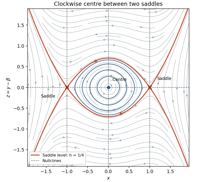
The phase plane in coordinates x and y minus beta, showing clockwise periodic orbits and saddle connections
. Details. 
Past exam of the differential equations 1 course of the University of Oxford 2021 3 a ii Solution 2026-10-25
Where , taking the quotient of the two ordinary differential equations givesChoose the first integralThe chain rule checks conservation even at points excluded in taking that quotient:Thus each trajectory is contained in a connected component of a level set of . At the gradient vanishes and the Hessian matrix is the identity, so has a strict local minimum there. To make the closed-trajectory argument explicit, put and . The bounded component of isThe two arcs join at to form a simple closed curve that is a regular level set. The gradient cannot vanish on it: the only critical point of a dynamical system in is the centre, whose level is .
The vector field is tangent and nowhere zero on this compact set, so its speed has a positive minimum. It therefore traverses the curve in finite time and returns to its initial point, giving a periodic orbit. These ovals shrink to the centre as . This is the planar first integral criterion for a centre and proves the required nonlinear assertion; it also gives Lyapunov stability without asymptotic stability.
Past exam of the differential equations 1 course of the University of Oxford 2021 3 a i Solution 2026-10-25
The equilibrium points satisfy and , so they areThe Jacobian matrix and its eigenvalue equation areAt the eigenvalues are , so both points are saddle equilibria. Their stable and unstable tangent directions have slopes and , respectively.
At the eigenvalues are , giving a centre for the linearized equation. Purely imaginary eigenvalues alone do not classify the nonlinear system. The first integral established in part (ii) proves that is in fact a centre equilibrium. It is clockwise: immediately to its right, with and , the vector field points downwards. Thus the final nonlinear classification is
Past exam of the differential equations 1 course of the University of Oxford 2021 2 c ii Solution 2026-10-25
Continuous dependence of an ODE solution on parameters here means continuity of the map into with its supremum norm: for every and , all sufficiently close satisfySubtract the two integral equations and use the uniform Lipschitz constant on the rectangle. With we obtainPart (i), with and , therefore proves, for ,The case follows from uniqueness or the same estimate with zero forcing. If , the direct integral estimate gives . In either case the map is even Lipschitz continuous, and hence continuous, throughout in the stated supremum norm.
Past exam of the differential equations 1 course of the University of Oxford 2021 2 c i Solution 2026-10-25
Treat both sides of at once: for set , . Nonnegativity givesDefine . By the fundamental theorem of calculus, and . The integrating factor givesSince , this proves the affine Gronwall estimate
Past exam of the differential equations 1 course of the University of Oxford 2021 2 b iii Solution 2026-10-25
Near the solution of a differential equation has , so the separable differential equation givesEquivalently its trajectory lies on the level setOn , the function is strictly increasing because , and its range is . Thus the positive branch exists exactly whereThe connected component containing isThe implicit function theorem gives a smooth solution of a differential equation at every such . It remains finite at every finite , because increases without bound. As , we have , and the original right side becomes singular. Hence this is the maximal interval through the prescribed initial condition.
In particular, the solution is not defined for all . It cannot pass through as a classical solution, since its required value there is .
Past exam of the differential equations 1 course of the University of Oxford 2021 2 b ii Solution 2026-10-25
The rectangle avoids the singular line exactly when . There , and the largest on is . Since decreases with , the smallest feasible uniform bound isIt is attained at , . For the Lipschitz constant, the mean value theorem givesThe quotients approach this upper bound as and , so the smallest feasible constant isSubstitution into part (a) givesThe contraction mapping restriction is automatic for every M-test-admissible precisely when . Because ,Thereforeis exactly the range where the two proofs guarantee all the same closed symmetric intervals, including the largest M-test interval.
For completeness, set and . The M-test allows ; the contraction mapping theorem allows with . At , these have the same supremum , but contraction excludes the endpoint . For , it gives the strictly shorter range . For a particular , both proofs work exactly when both displayed inequalities hold, even for these larger .
Past exam of the differential equations 1 course of the University of Oxford 2021 2 b i Solution 2026-10-25
With the standard constant starting Picard iterate, , the next two Picard iterates areand, for ,ThusThe restriction for is essential for the integral from to : the preceding iterate vanishes at , where the new integrand is undefined.
Past exam of the differential equations 1 course of the University of Oxford 2021 2 a 2 Solution 2026-10-25
For the direct contraction mapping theorem proof with the usual supremum norm, take the complete metric spaceand the Picard iteration map . The estimates areThus this proof requiresThe first inequality makes preserve ; the strict second inequality makes it a contraction mapping. Its unique fixed point is the desired solution of a differential equation.
This is more restrictive than the preceding Weierstrass M-test argument: a single application of must shrink every difference in the supremum norm, whereas repeated integration in the other proof produces the factorial and convergence even when . If , the additional condition is automatic. These are conditions for the two stated direct proofs; they are not necessary bounds on the actual existence interval.
Past exam of the differential equations 1 course of the University of Oxford 2021 2 a 1 Solution 2026-10-25
For the Weierstrass M-test proof of the Picard-Lindelöf theorem, the required bound isTo see this, use Picard iteration starting with andIf takes its values in , then . Thus every Picard iterate remains in the rectangle where the hypotheses hold. Successive applications of the Lipschitz condition and integration give the factorial estimate for Picard iterationFor example, the estimate is , and integrating the th estimate multiplied by proves the next one. The sum of the uniform bounds isfor every finite , by the exponential series. Hence the telescoping series of Picard iterates converges uniformly by the Weierstrass M-test. The uniform limit stays in the closed rectangle, and the Lipschitz condition permits passage to the limit in the integral equation. The fundamental theorem of calculus then gives the desired solution of a differential equation on .
Past exam of the differential equations 1 course of the University of Oxford 2021 1 c iii Solution 2026-10-25
The second-order differential operator factors asTherefore setting turns the second-order partial differential equation into exactly the first-order partial differential equation in part (a). Conversely, given a sufficiently smooth solution of a differential equation of that equation on a coordinate rectangle, defineThe fundamental theorem of calculus gives , so this solves the second-order equation, with an arbitrary twice continuously differentiable function . This classical correspondence is local on smooth patches; for the cornered solution of part (b), it can instead be interpreted using distributional derivatives.
Past exam of the differential equations 1 course of the University of Oxford 2021 1 c ii Solution 2026-10-25
For , the equation for the characteristic curves isThe two families are therefore and the characteristic projections from part (a), , together with the vertical characteristic . On either region or , the hyperbolic partial differential equation admits the characteristic coordinatesIndeed is constant along the first family, while . Their Jacobian determinant isThe coefficients of the two pure second partial derivatives in these coordinates vanish, and the coefficient of the mixed partial derivative is . Hence they give the hyperbolic characteristic normal form. They also remain regular at , provided .
The alternative , is valid on patches with . On , it is a parabolic partial differential equation away from the fully degenerate origin, so two independent hyperbolic characteristic coordinates are unavailable.
Past exam of the differential equations 1 course of the University of Oxford 2021 1 c i Solution 2026-10-25
In the convention , the coefficients of the principal symbol areThus the second-order partial differential equation isThere is no region of elliptic partial differential equation type. The terms hyperbolic, parabolic and elliptic refer to the pointwise classification of a second-order partial differential equation. At every second-order coefficient vanishes, so the principal symbol has rank zero and the equation is degenerate rather than genuinely parabolic there. Moreover the right side is , so no twice continuously differentiable classical solution can satisfy the equation at the origin.
Past exam of the differential equations 1 course of the University of Oxford 2021 1 b iv Solution 2026-10-25
For , . On the two sides of the corner-carrying characteristic curve, the partial derivative isAt every point with , the two one-sided partial derivatives are and . Therefore does not exist on this curve; its piecewise values have a jump discontinuity of magnitude . There are no other interior discontinuities. The values on the outer boundaries are interpreted from within .
This is exactly propagation of a derivative jump along a characteristic. Already on , the data have slopes and on the two sides of . The transport equation transports this corner along the characteristic curve from , which is ; it provides no smoothing. This is consistent with Noncharacteristic Cauchy data and does not contradict the smooth-data theorem, whose differentiability hypothesis fails here.
There are unlisted articles, also show them or only show them.