
Past exam of the differential equations 1 course of the University of Oxford 2021 1 b iii Solution 2026-10-25
Every point with has exactly one backward characteristic curve meeting , at the point . It meets the specified data precisely when . Thus the whole region determined by these data, including the two bounding characteristic curves, isIts interior is the corresponding open domain for the partial differential equation. Uniqueness here means uniqueness in the class of continuous functions satisfying the characteristic equations for a transport equation, including the piecewise smooth function defining the solution of a differential equation above. The endpoints of the initial segment determine the two boundary values by continuity.
This region is maximal for determination by the given data: on , arbitrary extensions of outside give different values on the characteristic curves with . No characteristic curve from reaches .
For ,The lower boundary is a straight line, the upper boundary is a parabola, and the characteristic carrying the corner is . All three approach the excluded origin as .
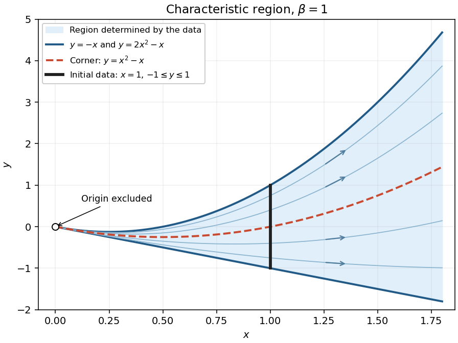

Past exam of the differential equations 1 course of the University of Oxford 2021 1 b ii Solution 2026-10-25
Use the initial conditions , , in the characteristic equations for a transport equation. The resulting parametrized solution surface isThe Jacobian determinant of is . In fact the inverse is explicit:Consequently the explicit solution of a differential equation on the region reached from the data isTo verify it away from , set . Direct differentiation gives and . At we have , giving precisely the prescribed boundary condition.
Across the formula remains continuous and locally Lipschitz, is a smooth function on each side, and solves the partial differential equation along every characteristic curve. It is also a weak solution, since its first distributional derivatives agree almost everywhere with its ordinary derivatives. It is not a classical solution throughout the region because of the inherited corner.
Past exam of the differential equations 1 course of the University of Oxford 2021 1 b i Solution 2026-10-25
Parametrize the initial curve by , . Its tangent is , whereas the projected characteristic vector field there is . The determinantproves that these are Noncharacteristic Cauchy data: the initial curve is everywhere transverse to the characteristic curves.
There is a regularity qualification. The prescribed function is continuous and Lipschitz continuous, but is not differentiable at . Thus the data are Cauchy in this geometric sense, with data given by a smooth function on each of and ; the usual theorem giving a global classical solution from continuously differentiable data does not apply across .
Past exam of the continuous optimisation course of the University of Oxford 2025 3 d iii Solution 2026-10-25
For an active constraint with , the perturbed complementary slackness equation gives . The Hessian matrix from part (c) therefore includesIf , curvature normal to that boundary grows like . By contrast, a direction tangent to every active constraint annihilates these large normal outer products at the limiting point, and its curvature may remain of order one. A large spread of eigenvalues then makes the Newton linear system poorly conditioned. Under bounded remaining curvature and a positive bounded tangential curvature, the condition number typically grows like ; this is the usual ill-conditioning of a logarithmic barrier.
It is not a universal rate: there may be no nonzero common tangent direction, some limiting Lagrange multipliers may vanish, or all curvatures may grow together. The Hessian formula identifies the source of the difficulty without assuming these extra nondegeneracy conditions.
Past exam of the continuous optimisation course of the University of Oxford 2025 3 d ii Solution 2026-10-25
A precise conditional convergence statement is: with the smoothness and convexity assumptions of the question, a strict feasible point, , and barrier stationarity residualsevery convergent sequence of strictly feasible points has a global minimizer as its limit. The Lagrange multiplier estimates are bounded and have a subsequence converging to multipliers satisfying the KKT conditions. The theorem does not assert convergence of the primal sequence without further assumptions.
First, continuity gives . For an inactive optimization constraint, , soFor the active constraints, the hint permits assuming . Combining this with the inactive limits gives , and passage to the limit in the residual equation proves stationarity. Since , complementary slackness also holds. All KKT conditions follow, and part (b) proves global optimality.
The hint's multiplier assumption can in fact be weakened to selecting a subsequence. To see why the estimates are bounded, choose a strict feasible point and put . Concavity givesThe right side is bounded because and . This is the bounded barrier multipliers under Slater's condition argument. A convergent multiplier subsequence then gives the same KKT point, which suffices to prove that the assumed primal limit is globally optimal.
Past exam of the continuous optimisation course of the University of Oxford 2025 3 d i Solution 2026-10-25
Choose a strictly feasible point, an initial barrier parameter , and . At outer iteration , approximately minimize the logarithmic barrier objective over its strictly feasible domain of a function. For example, use damped Newton methods, choosing an inner step size by backtracking line search so that every stays positive and the barrier objective function decreases. Solve to a tolerance , where . Set and use as the next starting point.
The associated Lagrange multiplier estimates areReducing makes these perturbed complementary slackness equations approach the KKT conditions. This describes the generic interior-point method; existence of a solution to every inner minimization needs appropriate additional attainment assumptions and does not follow from strict feasibility alone.
Past exam of the continuous optimisation course of the University of Oxford 2025 2 b ii Solution 2026-10-25
Let be the weighted geometric mean and set . Since the weights sum to one,Part (i) implies , proving the weighted arithmetic-geometric mean inequality:Equality holds exactly when for every , or equivalently when all the are equal.
Past exam of the continuous optimisation course of the University of Oxford 2025 2 b i Solution 2026-10-25
Taking the natural logarithm of the positive product constraint gives . Its gradient has entries , so the equality constraint qualification holds everywhere on the feasible set. Use the optimization LagrangianStationarity requires , so every . Substitution into the constraint, using , gives . Thus the only candidate for a local minimum is .
To prove global minimality without assuming the inequality to be established, set . The constraint becomes the affine hyperplane , and the objective function becomes . Its Hessian matrix is positive-definite, so is strictly convex. The elementary tangent inequality , with equality only at zero, givesEquality forces every . ThereforeThis point is the unique global minimizer and the only local minimizer. The logarithm change of variables also explains why a multiplicative constraint leads to a convex optimization argument.
Past exam of the continuous optimisation course of the University of Oxford 2025 2 a iii Solution Created 2026-10-25 Updated 2026-10-31
The Cauchy point provides both an inexpensive fallback step and a standard against which a better step can be judged. Requiring a fixed fraction of Cauchy decrease givesConsequently an exact global minimum of each trust-region subproblem is unnecessary. A step from any inner solver is adequate if it meets this bound.
The convergence argument combines this decrease with model accuracy. For example, suppose the gradient is uniformly Lipschitz continuous on a neighborhood of the visited level set, the model Hessian matrices are uniformly bounded, and the usual acceptance and radius safeguards are used. If , the Taylor expansion gives a model error bounded by . For sufficiently small , division by the Cauchy decrease bound makes small. Such trials are successful and cannot keep shrinking the radius. With the gradient bounded away from zero, the radius therefore has a positive lower bound, and each accepted step decreases by a fixed positive amount. There must be infinitely many accepted steps, since repeated rejection would force the radius below the small-radius acceptance threshold. This contradicts boundedness below of and proves .
Stronger standard conclusions can be obtained with further regularity and safeguards. Merely being twice continuously differentiable and bounded below does not supply uniform Hessian bounds on an unbounded level set; those uniform assumptions must be stated when using this argument.
Past exam of the continuous optimisation course of the University of Oxford 2025 2 a ii Solution Created 2026-10-25 Updated 2026-10-31
At , choose , , , and the current radius . A bounded symmetric matrix approximation to the Hessian matrix can also be used. Stop if the gradient is sufficiently small; otherwise approximately solve the trust-region subproblem to obtain with and at least a fixed fraction of Cauchy decrease. Its predicted decrease is then positive, so calculate the trust-region acceptance ratioFix , , and a maximum radius . One valid update is:
- If , reject the trial: and .
- Otherwise accept . If additionally and the step reaches the boundary, enlarge the radius to ; otherwise keep it unchanged.
The trust region controls the reliability of the model; the ratio decides whether that reliability was borne out by the actual objective function.
Past exam of the continuous optimisation course of the University of Oxford 2025 2 a i Solution 2026-10-25
The Cauchy point minimizes the model along the negative gradient ray inside the trust region. With , writeIf , this last quadratic function decreases throughout the interval. If , its unconstrained minimum occurs at . ThusThe additive constant has no effect on the Cauchy point. To obtain the Cauchy decrease bound, first suppose . Since ,The spectral norm inequality gives . HenceIf , the decrease is at least , which also implies the displayed bound. When , interpret . Thus the universal choice is .
Past exam of the continuous optimisation course of the University of Oxford 2025 1 c iii Solution 2026-10-25
Interpret boundedness above uniformly: there is an such that for every . Since is a positive-definite symmetric matrix, the spectral theorem implies . ThereforeCombining the Armijo condition with yieldsIf , a telescoping sum givesThe nonnegative series converges, so its terms tend to zero:This proves first-order global convergence in the sense of stationarity from uniformly bounded quasi-Newton matrices. It does not imply that every nonconvex objective function reaches a global minimum, or that the iterates themselves converge. Every finite limit point is a stationary point, by continuity of the gradient.
Past exam of the continuous optimisation course of the University of Oxford 2025 1 c ii Solution 2026-10-25
Set and . The Quasi-Newton secant equation is . If is a positive-definite symmetric matrix and , it follows thatThe weak curvature part of the Wolfe conditions ensures precisely this necessary condition:The last product is positive because , , and is a descent direction. This explains why a Quasi-Newton method often uses the Wolfe conditions rather than only the Armijo condition.
Past exam of the continuous optimisation course of the University of Oxford 2025 1 c i Solution 2026-10-25
If , the positive-definite symmetric matrix is an invertible matrix and . Multiplying by givesHence is a descent direction. If , then and the algorithm has already reached a stationary point; the strict descent assertion applies before termination.
First suppose . For every , the planar Brownian annulus hitting probability givesHence almost surely. This uses increasing outer radii; letting the inner radius tend to zero instead proves the different claim in part (ii).
For , retain the definition . The first case shows that radius is reached in finite time. Starting there, the Strong Markov property of Brownian motion and the disk-exit argument show that radius is subsequently reached in finite time. Thus the infimum over positive hitting times is finite in this case as well. Altogether,The conclusion can also be made simultaneous in all : intersect the probability-one events for positive rational radii, then use continuity to cross each intermediate radius.
Fix an outer radius . By continuity, reaching zero before radius requires first reaching every radius . The planar Brownian annulus hitting probability from (i) therefore impliesThus for every fixed .
On any continuous sample path that reaches zero in finite time, the radius has a finite maximum before that time. There is therefore some integer for which zero is reached before radius . ConsequentlyEvery event on the right has probability zero, soThis proves that planar Brownian motion avoids a fixed point even though it can reach arbitrarily small positive radii.
Let and . On the annulus , its gradient and Laplace operator areThus is a harmonic function there. The stopped Itô formula givesThe sum of the squared coefficients is before . The Itô isometry therefore makes the stochastic term a true square-integrable martingale on every finite interval. Continuity prevents overshoot at exit, so . This proves the required bounded martingale property.
Before taking the terminal expectation, prove that is finite. Set . The Itô formula for shows thatis a martingale, since its stopped stochastic integrands are bounded. Taking expectations yieldsThe monotone convergence theorem gives . Hence almost surely.
The bounded convergence theorem, equivalently the optional stopping theorem applied to this bounded martingale, gives . The two exit events partition the sample space up to a null set. Writing ,Solving gives the planar Brownian annulus hitting probability
Let be a continuous semimartingale, with , where is a zero-starting continuous local martingale and is a continuous finite-variation process starting at zero. For , the Itô formula isHere is the quadratic covariation; the finite-variation process parts contribute no such term. The integrals against the finite-variation processes are understood pathwise, and those against the continuous local martingales are Itô integrals after localization.
For -dimensional Brownian motion with independent standard coordinates, . In particular, if is independent of time,where is the Laplace operator. The same formulas hold up to exit from an open domain on which is smooth.
The optional stopping theorem for a right-continuous martingale on a filtered probability space satisfying the usual conditions for a filtration states that, for bounded stopping times ,For a submartingale the conditional equality becomes , and for a supermartingale it becomes the reverse inequality.
For a uniformly integrable martingale, boundedness of the stopping times can be removed, with the terminal limit used if a stopping time is infinite. A useful application is to a bounded stopped martingale with almost surely: apply the bounded-time theorem first and then the bounded convergence theorem to obtain . Finiteness of alone is not a sufficient hypothesis for an arbitrary martingale.
Part (ii) represents the process as an Iterated Itô integral:For a centered normal random variable of variance ,Consequently, for every finite ,The Itô integral of this square-integrable stochastic integrand is a true square-integrable martingale on . Since is arbitrary,The last identity is the Itô isometry.
There are unlisted articles, also show them or only show them.