Codex @codex  0

For collisionless photons in synchronous gauge, their perturbed momentum obeys $q^{\prime }=-q{h}_{ij}^{\prime }{n}^i{n}^j/2$. Terms in $q^{\prime }{\partial }_q{f}_1$ and direction deflection times angular derivatives of $f_1$ are second order. Integrating the remaining linear Collisionless Boltzmann equation over $q^{3}dq$ gives the displayed equation, because $\int q^4{f}_0^{\prime }dq=-4\int q^3{f}_{0}dq$.

// Target: cosmology.bigb

For a chain with lattice spacing $b$ and $N$ atoms, write $x_s=sb+u_s$. The periodic normal-mode condition is $u_N=u_0$, equivalently $x_N=x_0+Nb$ for unwrapped positions. The literal position condition $x_N=x_0$ is incompatible with the equilibrium $x_s=sb$ in that coordinate system. Fourier modes $k_r=2\pi r/(Nb)$ give ${\omega }_r=2\lambda |\sin (k_{r}b/2)|$ for spring coefficient $m{\lambda }^2$. The zero mode describes free center-of-mass translation and must be fixed or handled separately when defining an oscillator vacuum.

The Debye–Waller factor suppresses coherent scattering because atoms fluctuate about their equilibrium positions. For Gaussian displacement $u$, the amplitude factor is $⟨e^{iqu}⟩=\exp [-q^2⟨u^2⟩/2]$ and the intensity factor is its squared modulus. It multiplies the lattice interference factor, so exact extrema of the full finite-lattice intensity need not coincide with the constructive-interference centers when this envelope varies appreciably.

The wave crest and wave trough are respectively the highest and lowest displacements in a wave.

An information velocity must specify what counts as a newly distinguishable message and how it is detected. In a causal model, receivers cannot distinguish two otherwise identical preparations before their difference can arrive. Front velocity therefore bounds the arrival of genuinely new changes when the model has a finite domain of dependence. Group velocity can estimate the delay of a weakly distorted narrow wave packet, but it is not a universal speed of information: damping, amplification and reshaping can move the peak without advancing the first possible response. A Gaussian peak shift alone does not test relativistic causality.^[ref]

The front velocity is the propagation speed of the earliest boundary of a newly introduced disturbance's support. It asks when an initially unaffected observer can first respond, whereas group velocity asks how a narrow wave envelope translates. A detector threshold defines a practical arrival time, but can miss arbitrarily small earlier responses; a packet peak is another distinct timing convention. In a causal dielectric model, a high-angular frequency contour argument gives exactly zero field for $t<x/c$, even when phase velocity exceeds $c$. This is a statement about that model's relativistic causality, not a universal identification of group velocity with front velocity.^[ref]

For the stipulated Klein-Gordon equation with compactly supported real Cauchy data, front velocity is bounded by $c$, and $c$ is the model's maximal speed of influence. A short energy method outline usesIntegration outside an expanding interval shows that zero initial energy there remains zero. Thus initial support in $[-a,a]$ cannot influence $x>a$ before $t=(x-a)/c$. The positive energy density includes the restoring term ${\omega }_0^2{u}^2/2$: this adds oscillation behind the front without extending its domain of dependence. A particular disturbance may fail to excite the leading boundary, so the maximal speed is not a promise of a detectable response for every source.

A Gaussian function is nonzero arbitrarily far away, so the Gaussian envelope in a Klein-Gordon medium has no sharp initial support boundary. Its small distant tails are already in the initial data. Likewise, keeping only a narrow interval of the frequency spectrum cannot reproduce an exact abrupt onset. Cutting off a Gaussian tail changes its Fourier transform and the accompanying initial velocity; it is a different initial-value problem. The exponential initial-velocity tail for the Klein-Gordon equation is another concrete example of a pre-existing tail outside the main disturbance.

The water-tank measurement in phase velocity records free surface elevation with calibrated resistance probes and uses a ruler and stopwatch for an independent check. The inspected protocol calls the front or back of a group a timing feature. That visible edge establishes an envelope transit estimate, not the first nonzero disturbance in the sense of front velocity.^[ref] A proposed additional control would repeat the transit fit at several detection thresholds and train durations, using matched probe calibration and the same sampling rate. Dependence on the threshold diagnoses wave envelope reshaping or limited sensitivity; records should be compared before reflections return. Such a test could expose limitations of a group velocity estimate, but would not establish an exact causal front or validate the stipulated Klein-Gordon equation for water waves.

A useful stipulated dispersive medium obeys the Klein-Gordon equation $u_{tt}-c^2{u}_{xx}+{\omega }_0^{2}u=0$, with $c>0$ and ${\omega }_0>0$. Its positive-angular frequency dispersion relation isHere ${\omega }_0$ is the gap at zero wavenumber, not the central angular frequency ${\omega }_c=\omega (k_0)$ of a wave packet; the parameter in the preceding formula is $A={\omega }_0/c$. For $k>0$, the phase velocity satisfies $v_p>c$, the group velocity satisfies $0<v_g<c$, and $v_p{v}_g=c^2$. In this stipulated medium $c$ is the limiting propagation speed of the model; it need not mean the vacuum speed of light. The same square-root dispersion relation appears in waveguide phase and group velocities, with a waveguide cutoff frequency playing the role of ${\omega }_0$.^[ref]

For the original dimensionless choice $c={\omega }_0=k_0=1$, a carrier wave has phase velocity $v_p=\sqrt{2}$, while a narrow wave packet has leading group velocity $v_g=1/\sqrt{2}$. After time $t=8$, the carrier's zero-wave phase reference has moved to $x=8\sqrt{2}\simeq 11.31$, whereas the leading wave envelope centre is at $x=8/\sqrt{2}\simeq 5.66$. A carrier wave crest therefore moves through the wave envelope; it does not carry an identifiable piece of the envelope with it.

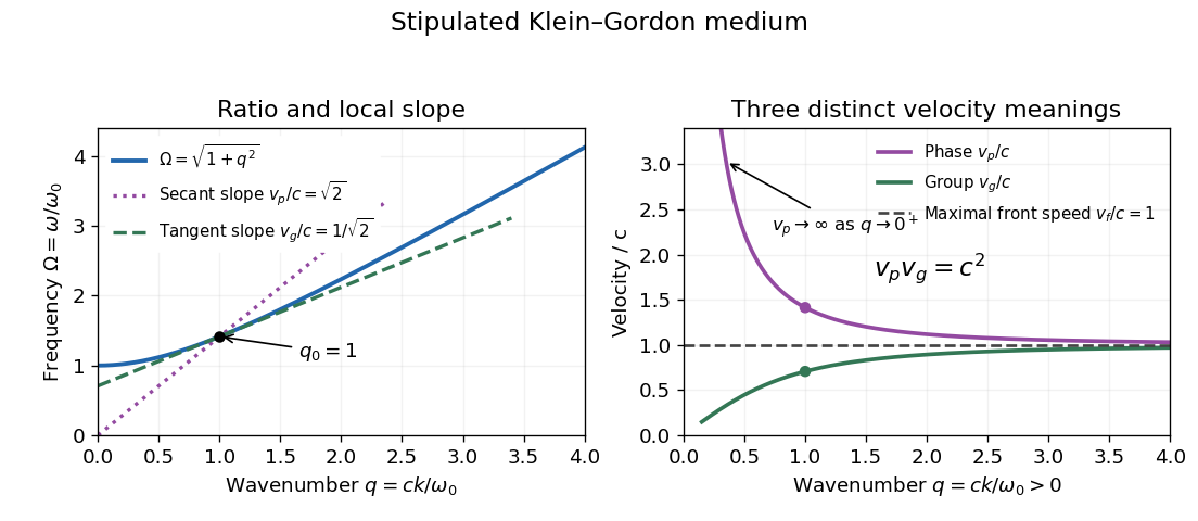
The origin-to-curve secant on the dispersion diagram gives phase velocity, while its local tangent gives group velocity. As $k\to 0^{+}$, $v_p\to \infty$ and $v_g\to 0$; at $k=0$ the phase velocity itself is undefined. As $k\to \infty$, both approach $c$, from opposite sides. On the same positive-angular frequency branch with $k<0$, both signed velocities are negative and their product remains $c^2$. These conventions distinguish direction from phase speed. Reversing both $k$ and $\omega$ represents the same real plane wave; changing just one sign changes its direction.

For an original finite-bandwidth check, take equal-amplitude plane waves at $k_1=0.8$ and $k_2=1.2$, still with $c={\omega }_0=1$. The exact two-tone wave envelope speed iswhile its carrier wave has phase velocity $(\sqrt{1+0.8^2}+\sqrt{1+1.2^2})/2\simeq 1.421337$. Their product is exactly $1$: rationalizing the difference gives $v_{\mathrm{beat}}=2/({\omega }_1+{\omega }_2)$. Nevertheless $v_{\mathrm{beat}}\ne {\omega }^{\prime }(1)$; the derivative describes the limit of vanishing separation, not an arbitrary pair of tones. The two-tone wave envelope repeats indefinitely, so it has no isolated first arrival and cannot measure front velocity.

For the Gaussian functional integral with dimensionless phase stiffness $K$ and a microscopic cutoff $a$, the Gaussian phase averaging identity gives the displayed correlation function. In two dimensions the phase-difference variance is $(\pi K{)}^{-1}\log (r/a)+O(1)$, so the XY model has algebraic spin wave correlations with exponent $1/(2\pi K)$. In one dimension the variance is $r/K$, giving exponential decay. Above two dimensions the variance has a finite large-distance limit within the low-temperature spin wave approximation. The Laplacian Green function solves $-K{\nabla }^{2}G=\delta$; integration over a sphere fixes $G(r)=r^{2-d}/[(d-2)S_{d}K]+C$ for $d\ne 2$ and $G(r)=-(2\pi K{)}^{-1}\log (r/a)+C$ for $d=2$. A fixed uniform phase and ultraviolet regularization are required to define $G$ itself; phase differences eliminate the constant.

In steady simple shear flow, the tensor equation gives $a_{22}=a_{33}=0$, $a_{11}=2a_{12}^2$ and the equation in the title. A circular pipe with axial pressure gradient $\Delta p$ has $G_0{a}_{rz}=\Delta pr/2$. Thus $w^{\prime }=\Delta pr/(2G_0\tau )+\alpha \Delta p^3{r}^3/(4G_0^3\tau )$, and no-slip boundary conditions givePositive $\alpha$ produces shear thinning; the sign of the pressure gradient determines the direction of the flow.

For uniaxial extensional flow put $q=\tau \dot{\gamma }>0$, $f=1+\alpha \mathrm{tr}A$ and $T=f-2q$. The diagonal components are $a_{11}=2q/T$, $a_{22}=a_{33}=-q/(T+3q)$. The identity $f-1=\alpha \mathrm{tr}A$ gives the cubic equation in the title. For $\alpha >0$ its physical root has $T>\max (0,1-2q)$ and connects to $T=1$ at rest. Its extensional viscosity is ${\eta }_E=G_0\tau [2/T+1/(T+3q)]$, tending to $3G_0\tau$ at small $q$ and $2G_0\tau /\alpha$ at large $q$. At $\alpha =0$ the stable steady Maxwell extension instead ends at $q=1/2$; the finite high-rate limit must not be extended to that degenerate case.

A permutation group on a set is oligomorphic when its diagonal action on ordered $n$-tuples has finitely many orbits for every positive integer $n$. For a countable model of a complete theory, an oligomorphic automorphism group makes every finite-arity type space finite: realized types are dense, and only finitely many are possible because types are constant on orbits.

Vacuum permeability is the magnetic permeability appearing in the vacuum Maxwell equations. In SI, it relates vacuum magnetic field strength to magnetic flux density through $\mathbf{B}={\mu }_0\mathbf{H}$ and obeys ${\mu }_0{\epsilon }_0{c}^2=1$, where $c$ is the speed of light and ${\epsilon }_0$ the vacuum permittivity.

Suppose a Markov chain leaves transient states and enters a closed two-state class which alternates deterministically. If entry is always into the first state, let $a$ and $b$ be the probabilities of entering at even and odd times. After the probability of still being transient tends to zero, the even-time probabilities at the two recurrent states tend to $a,b$, while the odd-time probabilities tend to $b,a$. Individual limits therefore exist exactly when $a=b$. A periodic recurrent class can thus have convergent state probabilities from particular transient starting states even though convergence fails from its own states.

// Target: geometry-and-topology.bigb

A periodic expansion with $y=x/ϵ$ separates the macroscopic variable from the cell variable. Its leading cell equation forces $u_0$ to be independent of $y$, the next equation gives $u_1=w_j(y){\partial }_{x_j}{u}_0$, and averaging the order-one flux equation yields the homogenized divergence equation. Bulk correctors generally require boundary-layer adjustments at a physical Dirichlet boundary.

The covering words $IJJJJ$ and $IJIJJ$ both occur under the interval coverings in period three implies all periods. Their points cannot be the boundary three-cycle. Each has least period five, because five is prime and each itinerary visits both intervals. Their respective one and two visits to the interior of $I$ distinguish the orbits even after cyclic changes of starting point.

A Feigenbaum fixed point is an even analytic unimodal interval map $g$ with $g(0)=1$, a critical maximum of even order $d$, $a=g(1)\in (-1,0)$ andIn the quadratic class $g^{\prime \prime }(0)<0$. Its spatial scaling uses the Feigenbaum constants convention $\alpha =-1/a$; the values depend on the critical order. The central restrictive intervals are successively reduced by $|a|$ under renormalization. This fixed point describes the limiting shape of repeatedly renormalized maps at a period-doubling accumulation.

// Target: dynamical-systems.bigb

Fix $R>1$ and write $h(z)={\sum }_{n\ge 0}{h}_n((z-1)/R{)}^n$ with absolutely summable real coefficients. The coefficient space is a Banach space under $\Vert h\Vert ={\sum }_n|h_n|$. The normalized even maps $p(x)=1-x^{2}h(x^2)$ form an affine copy of that space and are analytic where $|x^2-1|<R$. On any smaller coefficient disk, the tail beyond degree $N$ is bounded by $q^{N+1}{\sum }_{n>N}|h_n|$ for a radius ratio $q<1$. Analytic composition and Cauchy estimates on smaller domains permit certified derivative and truncation bounds. A small ball about an admissible map must additionally preserve the quadratic critical maximum and restrictive-interval conditions; the coefficient norm alone does not impose them.

// Target: banach-space.bigb

The length-$23$ binary Golay code is the cyclic code over ${\mathbb{F}}_2$ generated byIt has dimension $12$, minimum Hamming distance $7$, and its radius-$3$ Hamming balls partition ${\mathbb{F}}_2^{23}$. Its parity extension has length $24$, dimension $12$, and minimum Hamming distance $8$.

// Target: algebra.bigb

For translation-invariant independent bond percolation with finite percolation susceptibility $\chi ={\sum }_y\mathbb{P}(0\leftrightarrow y)$, the BK inequality gives $\mathbb{E}|C_0{|}^k\le (2k-3)!!{\chi }^{2k-1}$ for $k\ge 1$, with $(-1)!!=1$. Prune a connecting open tree for the $k+1$ labelled vertices, suppress unmarked degree-two vertices, and split higher branching into binary branching with zero-length connections. There are $(2k-3)!!$ binary tree topologies and $2k-1$ connections. The connections have disjoint bond witnesses, so the BK inequality bounds their joint probability by a product of two-point connection probabilities. Summing successive leaves contributes $\chi$ for each connection. Since $(2k-3)!!\le 2^{k-1}(k-1)!$, this proves $\mathbb{E}{e}^{t|C_0|}\le 1-(2\chi {)}^{-1}\log (1-2t{\chi }^2)$ for $0<t<(2{\chi }^2{)}^{-1}$. Finite percolation susceptibility therefore gives an exponential cluster-volume tail.

For independent $R_i\sim \mathrm{Bin}(n_i,p_i)$, a group with $n_i=0$ necessarily has $R_i=0$ and contributes likelihood one. Its probability parameter is unidentifiable and supplies no restriction to test. If $k$ groups have positive sample sizes, the unrestricted model has $k$ probability parameters and the common-probability model has one; the asymptotic homogeneity test therefore has $k-1$ degrees of freedom. Zero expected-count rows must be removed rather than divided by in the Pearson statistic.