
Non-Archimedean part of Ostrowski theorem 2026-10-14
For a nontrivial Non-Archimedean absolute value on , every integer has absolute value at most one. Some prime must have value less than one, or the value would be trivial on every rational number. Two distinct such primes are impossible by a Bezout identity. Prime factorization then gives the displayed formula. Distinct primes give inequivalent topologies, since powers of tend to zero only for the -adic absolute value among these values.
Osmosis concentration-pressure example 2026-10-14
Take two reservoirs separated by a semipermeable membrane that passes water and retains one neutral solute. Stipulate , and , equivalent to and . Treat both chemical solutions as dilute and ideal. These are invented model conditions, not measurements or recommended biological conditions.
For pressures measured at the same height beside the membrane, define . The model predictsAt , net water transfer favors A to B. At , the opposing pressure balances the osmotic pressure difference, giving zero net transfer with unequal concentrations. At , the sign reverses and net water transfer favors B to A, toward the more dilute reservoir. Raising pressure changes the total water potential, rather than changing the membrane into a one-way gate.
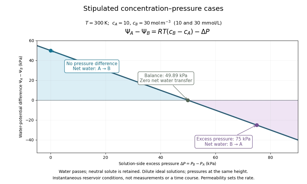

Fixed concentrations require large maintained reservoirs or an instantaneous comparison. In a closed membrane osmometer, entering water causes dilution of the receiving chemical solution and changes its volume; the final balance must use final concentrations. A supported cell wall provides another way to develop the opposing pressure, as explained under turgor pressure.
Astrocentric osculating-element oscillations 2026-10-14
A circular distant barycentric Kepler orbit around a circular star–planet binary need not have constant star-centred osculating orbital elements. Let be the planet's fraction of the binary mass, , and . Subtracting the stellar reflex velocity produces radial and tangential perturbations , where is the planet's longitude minus the particle's longitude. The vis-viva equation gives the displayed semi-major axis variation. The eccentricity vector components follow from and . The errors are ; the spatial translation itself is only . These are changes of instantaneous orbital description, even when the assumed barycentric trajectory is fixed.
Tensor products of the assigned vectors represent strong graph powers, and tensor products of the handle have squared inner products equal to products of the original ones. The vectors assigned to an independent set are orthonormal. Bessel inequality then bounds its size by the largest inverse squared handle inner product. Taking roots and minimizing proves .
Oriented frame bundle of de Sitter spacetime 2026-10-14
Represent unit-radius de Sitter spacetime by the spacelike unit hyperboloid in five-dimensional Minkowski spacetime. Appending its position vector as the last column of an oriented pseudo-orthonormal frame produces a matrix in . Projection to that last column identifies with the oriented orthonormal frame bundle, a principal bundle with group . The full bundle allowing both orientations is with group . Requiring a time orientation as well selects the corresponding identity components.
An oriented pseudo-orthonormal frame in Minkowski spacetime consists of its base point and a Lorentz matrix acting on a fixed reference frame. The pairs form the Poincaré group, and right multiplication by sends the frame to while fixing its base point. Thus the displayed projection is a principal bundle with group . The full frame bundle uses ; a specified time orientation restricts to the corresponding connected component.
Represent the Anti-de Sitter spacetime quadric by in . Appending its timelike unit normal to an oriented tangent pseudo-orthonormal frame identifies the frame bundle with . The stabilizer of that normal is , so projection realizes as the base of a principal bundle. For the commonly used universal cover of the anti-de Sitter quadric, pull this bundle back along the covering map; the quadric itself has a periodic timelike coordinate.
Integrated Ornstein-Uhlenbeck displacement 2026-10-14
For a thermal inertial Langevin equation conditioned on fixed initial position and velocity, the centered displacement is . With the fluctuation-dissipation relation for a Langevin particle, and integrating the squared kernel gives the displayed variance. At short times it is per component; at long times it is . Averaging initial velocity over thermal equilibrium adds a ballistic contribution and gives per component.
Let , , and , . The logarithm is a centered Gaussian random variable of variance . Squaring the stochastic kernel and integrating proves this formula. The exponential moment of a Gaussian linear functional gives and the displayed long-time growth exponent. Positive moment growth with zero mean strain reflects the breadth of the log-normal distribution; it does not imply positive growth of the mean logarithm.
The linear stochastic differential equation has the explicit solution . Its integrating factor is . For , an independent initial normal variable of variance makes its zero-mean Gaussian process stationary.
For , set and . This is a Brownian motion in the new filtration; its independent Gaussian increments have variance equal to elapsed time. The Itô product rule gives . Its initial value is , independent of future W increments, and its covariance function is . Consequently it is a stationary Ornstein-Uhlenbeck process. The quadratic variation of the unscaled time change is , not .
Stationary drift saturation 2026-10-14
For an adapted stationary process with the displayed bounds, the Itô formula and stationarity give . The Cauchy-Schwarz inequality makes each integrand nonnegative, so equality holds almost everywhere. Then , proving for almost every time and outcome. Thus the process solves the Ornstein-Uhlenbeck stochastic differential equation and its initial value, rather than stationarity alone, determines its coupling with W.
For any step , set . The Ornstein-Uhlenbeck transition distribution gives the exact updateusing a fresh independent standard normal random variable for each interval. The update reproduces the joint probability distribution on the selected time grid. It can start from a fixed value or use Ornstein-Uhlenbeck stationary initialization. On an equally spaced grid it is an autoregressive process of order one after subtracting . Its stationary variance follows directly from .
For the stipulated example with , and the innovation variance is . Given , the next conditional expected value is about and the conditional standard deviation is about .
The Euler-Maruyama method instead approximates the same stochastic differential equation byFor its stationary variance solves , givingAt in the example, this is , about above the continuous model's stationary variance. If , this Euler recurrence has no finite stationary variance despite the stable continuous model. Exact transitions avoid this discretization error at sampled times; neither update alone determines the unresolved motion between samples.
Ornstein-Uhlenbeck stationary initialization 2026-10-14
Set and draw independently of future Brownian increments. The Ornstein-Uhlenbeck process is then a strictly stationary process, withEvery time has the same normal distribution, and the covariance function depends only on the time lag. For a Gaussian process these properties also make all its finite-dimensional distributions invariant under a common time shift. The stationary distribution balances the continual random forcing against the contracting drift.[ref]
Applied Stochastic Differential Equations by Simo Särkkä and Arno Solin. Applied Stochastic Differential Equations, Example 6.8, printed pp. 91–92, equations (6.73)–(6.76): steady-state variance and covariance
With a fixed , the covariance function instead isIn particular, it is zero when , since the initial value has no uncertainty. The second term records the fixed start; it is the general scaling of the zero-start Ornstein-Uhlenbeck covariance. The pure exponential covariance function displayed above assumes stationary initialization. For a fixed start, that function emerges as the late-time limit at fixed lag, while the one-time probability distributions approach by convergence in distribution.
For the stipulated , , , stationary initialization has variance one from the outset. Its autocorrelation is , so the correlation time is one: a lag of one reduces the autocorrelation to . Its raw second moment includes the squared expected value; it must not be confused with the covariance.
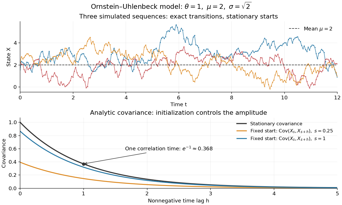
Simulated stationary Ornstein-Uhlenbeck samples and analytic covariance compared with a fixed start
. Details. 
The upper panel shows three simulated sequences with independent stationary initial values and exact transitions at spacing . Joining their points only guides the eye; it does not simulate a continuous sample path between those points. The lower panel shows analytic covariance functions: the stationary curve and, for comparison, for fixed initialization at two different ages . These are simulated samples and model curves, not measured trajectories or empirical covariance estimates.
Ornstein-Uhlenbeck transition distribution 2026-10-14
For a fixed initial value , the Ornstein-Uhlenbeck process has the normal distributionThe two parameters of are the expected value and variance, not the standard deviation. At the variance is zero and the value is fixed. More generally, its transition kernel over any interval of length has conditional expected value and conditional variance when the current value is . The coefficients depend on elapsed time; the initial probability distribution determines whether the resulting stochastic process is stationary.[ref]
In the stipulated example , , , , the expected value at time two is and the variance is . The initial distance from two has fallen by a factor , but the standard deviation has grown to about . Approaching the reference level in expected value is compatible with growing uncertainty from a perfectly known initial value.
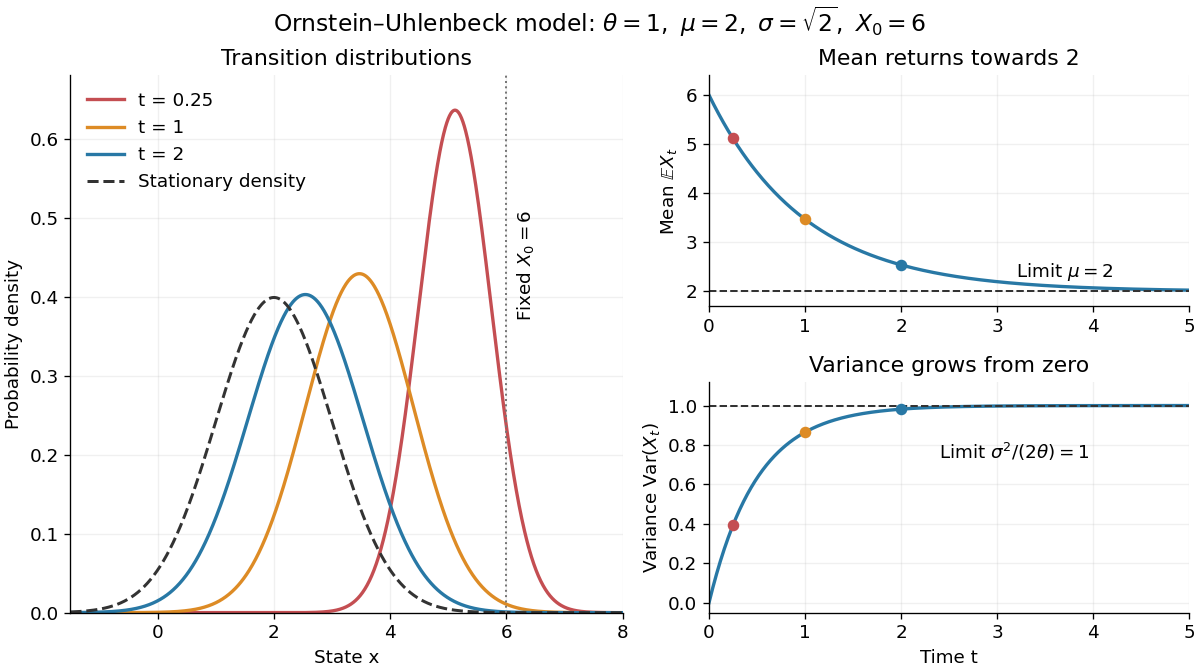
Ornstein-Uhlenbeck transition densities, mean relaxation and variance growth from a fixed initial value
. Details. 
The solid probability density functions use times , and ; the dashed curve is the limiting normal distribution with expected value two and variance one. The curves are exact model predictions. There is no ordinary density for the fixed value at time zero.
A short derivation uses the integrating factor . The Itô product rule gives , henceThe stochastic integral has zero expected value. The Itô isometry gives its variance as . Its deterministic integrand makes it a Gaussian random variable, yielding the displayed normal distribution. Shifting the integration interval gives the same transition kernel from any later time.
Orientability of a vector bundle total space 2026-10-14
The total space of a real vector bundle has the exact sequence . Taking determinant line bundles gives the displayed identity. If is an orientable smooth manifold, the total space is orientable exactly when is trivial. Sufficiency follows by pullback; necessity follows by restricting the total-space determinant identity to the zero section. For the cotangent bundle, base and fibre coordinate determinants cancel, giving an orientation even when the base is not orientable.
Rank of a well-founded tree 2026-10-14
The rank of a terminal node is zero; the rank of any node is the supremum of the successor ranks of its immediate extensions. The rank of the empty node gives one convention for tree height. Every countable well-founded tree has countable rank. Changing between empty-root rank and successive leaf-deletion order changes harmless endpoint conventions.
Coordinate vector 2026-10-14
For an ordered basis , the coordinate vector records the unique coefficients satisfying . Change of basis changes this representation while preserving the underlying vector.
For , , the vector has coordinate vector , since . These are the same coefficients extracted by the dual basis in its worked example. The vector is independent of the chosen basis; its list of coordinates is not. In an orthonormal eigenbasis, the coordinates additionally separate the action of a self-adjoint operator into independent scalar multiplications.
Give the lexicographic order and the order topology. Every point has an interval neighbourhood between and , lying entirely in the vertical line . These intervals give each such line its usual real topology, and every line is open. Thus this space is a disjoint union of uncountably many open copies of the real line and is not a second-countable space: any basis of a topology must supply a different member inside each of these disjoint nonempty open sets.
Strict order-preserving function 2026-10-14
A strict order-preserving function preserves strict comparisons. Between strict partial orders it may identify incomparable elements. Between strict total orders it is necessarily injective, and in a finite chain it is exactly an increasing injection. It need not reflect comparisons between incomparable elements of general partial orders.
There are unlisted articles, also show them or only show them.