
Complete the square in the Fourier transform exponent:The supplied shifted Gaussian integral therefore givesThis is the Fourier transform of a Gaussian, with angular-wavenumber convention .
Take the spatial Fourier transform of the heat equation. Two integrations by parts, with decaying fields and first derivatives at infinity, give . Thus each mode satisfies the ordinary differential equationInserting the transformed initial condition and integrating the time equation givesFinally set . The inverse Fourier transform, evaluated by the same Gaussian identity, givesEquivalently the Gaussian initial data for the heat equation evolve asThe profile broadens and its peak decreases, while its total integral remains , as required by diffusion without loss on the whole line. Direct differentiation verifies the equation and the initial limit.
The homogeneous equation is a Cauchy-Euler equation. Trying gives the repeated indicial rootHence, for ,Both independent solutions diverge at the origin, so no nonzero homogeneous combination satisfies the zero-origin conditions by continuous extension.
For a source point , finiteness on forces the Green function to vanish on that side. On , continuity and the unit first-derivative jump requireUsing the homogeneous solutions gives the causal Green function for a repeated-root Euler operatorIndeed, the Wronskian of and is , and direct differentiation gives . Since is continuous, its second derivative produces precisely a unit Dirac delta, with no derivative of a delta. For each positive source it is identically zero near the origin, so both required origin values vanish. The differential operator itself is interpreted on ; no value of its singular coefficients at zero is needed.
Integrating against the forcing yieldsThe last integral equals , by integration by parts or differentiating . ConsequentlySubstitution gives , while . The divergent homogeneous solutions prove uniqueness in the regular class. No boundary condition at infinity was imposed or required.
For a spherically symmetric number density, the radial Laplacian is . Applying separation of variables and choosing the separation constant givesso the ordinary differential equations areThe radial problem is an eigenvalue problem for with Dirichlet boundary conditions, hence : multiplying the radial equation by and integrating gives for a nonzero regular mode vanishing at .
To solve it explicitly, set , corresponding to the suggested power . The equation reduces to , soFiniteness at the origin forces , and the Dirichlet boundary condition at requires for an integer . The absence of interior zeros excludes , selecting the fundamental normal mode. If denotes the initial central density, the result iswhere the sine ratio is defined as at the origin. It is strictly positive in the interior for every finite time. The arbitrary positive scale cannot be fixed without additional initial data.
The spatial factor is time independent, so the density and the total neutron population have the same exponential growth rate. Thus the spherical reaction-diffusion growth threshold isAt equality the fundamental mode is stationary; below it the mode decays. For fixed , the equivalent critical-radius condition is . This is the competition between multiplication in the bulk and diffusion loss at the surface in the stated dimensionless model.
Using Cartesian coordinates, the Levi-Civita symbol and the Einstein summation convention, the constant-vector assumption givesRecognizing the divergence and directional derivative provesHere the contractions use the Kronecker delta.
For an oriented piecewise smooth surface with boundary , Stokes theorem stateswhere the orientations obey the right-hand rule and is continuously differentiable near . Apply it to . The scalar triple product givesThe last integrand is , as the component formulashows. Since is arbitrary, the cross-product form of Stokes theorem follows:The derivatives in the surface expression act on , not on the surface element.
For the specified square, the path is clockwise when viewed from positive , so the compatible unit normal is . On the first and fourth edges, and are parallel, giving zero cross product. On the second edge, and runs from to , so contributes . On the third edge, and runs from to , so the contribution is . Thus the line integral is .
For an independent surface integral, and for the position vector field. Its integrand is therefore . The square has unit area and downward orientation, giving
The intersection contains the identity element. If , then belongs to both and , so it belongs to their intersection. The subgroup test proves that is a subgroup of , with the inherited operation. Explicitly, closure and inverses come from this test, and associativity is inherited from .
Label the vertices of the equilateral triangle counterclockwise. For the dihedral group of order six, let be the counterclockwise rotation by , and let be reflection in the line through vertex 1 and the opposite side's midpoint. ChooseThen rotates by . The three Euclidean reflections fix vertices respectively. Products act on a vertex from right to left. The relations and givewhere exponents of are reduced modulo three and those of modulo two. This constructs the entire Cayley table:For example whereas , so the group is nonabelian.
A subgroup of order two is generated by its unique nonidentity element, which must have order two. The rotations have order three, and each reflection has order two. Thus there are exactlyNone is a normal subgroup. Conjugation by sends the reflection to , cycling the three reflections. For example . Each of the other two subgroups fails the same conjugation test.
The group order of a finite group is its number of elements, . The order of a group element is the least positive integer with . Such an exists in a finite group because two powers must coincide, and cancellation then gives a positive power equal to the identity element.
For the direct product of groups, the componentwise operation is closed because each factor is closed. Associativity holds in each coordinate:The identity element is , and the inverse element of is . Thus all group axioms hold. For finite factors, the multiplication principle gives
For , write , , , , with . Its Cayley table, with the row element multiplying the column element, isThis is the Klein four-group: every nonidentity element has order two.
In the cyclic group , the set is closed because , and both elements have inverses in the set. It is therefore a proper subgroup of order two. By Lagrange's theorem, a proper subgroup has order one or two. An order-two subgroup must be generated by an element of order two. Neither nor has order two, whereas does. HenceThe PDF's claim needs “nontrivial”: is the only nontrivial proper subgroup, but is also a proper subgroup under the usual definition.
A group isomorphism preserves element orders: if and only if , using the homomorphism property and injectivity. Since has elements of order four and the Klein four-group does not,
The Lagrangian is , and the Euler-Lagrange equations areAt a rest equilibrium , for all three coordinates. The Taylor expansion therefore starts asThe symmetric Hessian matrix is the matrix of the quadratic potential energy. If a quadratic coefficient vanishes along a direction, higher-order terms can be the first nonconstant terms there; equilibrium by itself does not imply strict stability.
Write . Terms involving the variation of are cubic in small displacements and velocities, so the quadratic small oscillation Lagrangian isA normal mode has fixed displacement ratios, . Its angular frequency is an eigenfrequency, or normal frequency, and satisfies the generalized eigenvalue problem for small oscillationsHere is positive definite for independent physical coordinates and positive masses. A stable quadratic minimum makes ; a negative value would describe exponential instability rather than oscillation.
For the suspended bar, let and denote the actual incremental spring constants of the upper and each lower spring. The physical displacement of the bar is , while the lower spring extensions change by and . ConsequentlyThe linear gravitational and elastic terms cancel at the loaded equilibrium. Expanding the remaining squares gives the small-oscillation mass and stiffness matricesThusSource convention: the printed matrix is obtained by setting and . Although the PDF prose calls spring constants, that matrix treats them as elastic parameters whose ratios to the stated lengths are the incremental stiffnesses. If they are read literally as Hooke-law spring constants, the divisions by should instead be omitted. The numerical case has , so this discrepancy does not affect its results.
With the numerical parameters, andUse the exchange symmetry of the lower masses to find the vertical modes of a horizontally constrained suspended bar. The antisymmetric vector obeys , giving . In the symmetric sector put and . The two independent equations areTheir determinant gives , so . Taking , the full set isIn the lowest normal mode, all three masses move in phase, with the lower masses moving about times as far as the bar. In the antisymmetric normal mode, the bar stays still and the lower masses move equally in opposite directions; their changing forces on the bar cancel. In the highest normal mode, the lower masses move together against the bar, with magnitude about of its displacement. Any small motion is a superposition of these three modes.
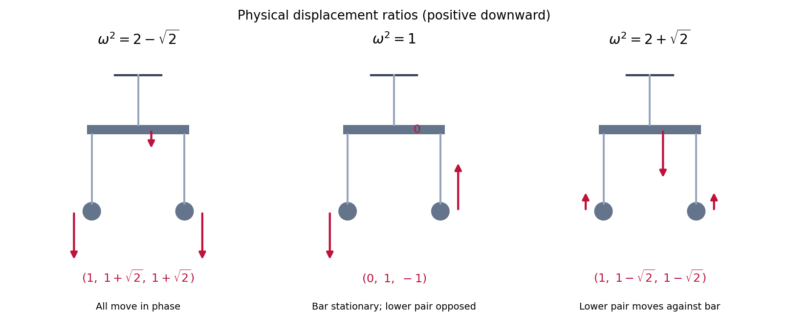
Relative vertical displacements in the three normal modes, with the bar constrained to remain horizontal
. Details. Let be the orthogonal matrix taking old components to new ones, so . With repeated indices summed, the tensor component transformation law isAn isotropic tensor has the same components after every proper rotation. Since , the Kronecker delta is invariant. Applying this identity to each factor shows that and every linear combination are invariant as well.
To show that an isotropic second-rank tensor must be scalar, start with any matrix , without assuming symmetry. Invariance under quarter-turns about axes 1 and 2 implies invariance under their squares, the half-turnsThe first forces to vanish. The second also forces to vanish. The matrix is therefore diagonal. A quarter-turn about axis 1 interchanges its 22 and 33 entries; one about axis 2 interchanges its 11 and 33 entries. All three must agree, giving .
A rotation preserves the ball , and the volume element. Changing integration variables by that rotation shows that and are isotropic tensors. Write . Taking its tensor contraction givesso . Every permutation of the indices of leaves its integrand unchanged. Its complete symmetry therefore makes all three isotropic coefficients equal, say :Double contraction gives . Thus the isotropic fourth moment of a ball and its radial contraction are
Put , so that . Contract with the prescribed unit vector twice:This has the spectrum of a scalar matrix plus a rank-one projector. In the direction , the outer product acts as the identity; on the plane perpendicular to , it acts as zero. ThereforeAny nonzero multiple of is a parallel eigenvector, and any nonzero vector in the perpendicular plane is a transverse eigenvector. The transverse eigenvalue has multiplicity two; an orthonormal basis of that plane completes a set of principal axes.
First prove the convolution theorem with the stated negative-exponential Fourier transform. Assuming absolute integrability sufficient for Fubini's theorem, change variables :
For the differential equation, integration by parts givesThe boundary terms vanish by the assumed decay of . As with the convolution step, the transforms can first be justified for integrable functions and derivatives; the resulting kernel gives the desired decaying response. ThusThe convolution theorem and Fourier inversion theorem imply .
For the inverse transform of , useThe poles are at . For , close the inverse-transform contour above; the residues of there are and . The inverse-transform factor makes the answer times their sum. For , close below, enclosing no poles. The large arcs vanish: the complete rational factor is and the exponential is bounded on the appropriate semicircle. Therefore the causal Green function of an overdamped oscillator isIt is continuous, with and , so . The response can also be written .
For the bilateral exponential forcing, split the real integral at zero:ConsequentlyFor negative time the lower half-plane contains only . The residue of there is . Clockwise closure makes the inverse transform times that residue. For positive time the three upper residues, at respectively, areMultiplication of their sum by gives the bilateral exponential forcing of an overdamped oscillator:Both expressions have . This verifies the matching that prevents an extra Dirac delta function at zero. Direct substitution gives the forcing on either side, and all terms decay at their corresponding infinities. A causal Green function does not imply zero response before when the forcing has already been acting at negative times. The assumptions avoid repeated poles; their limiting cases would contain polynomial times exponential terms.
For a positively oriented simple closed contour , with no pole on and with holomorphic inside except at finitely many poles, the residue theorem statesFor a more general closed contour, each residue is multiplied by its winding number about the pole.
The powers must be defined using the same branch of the complex logarithm as the numerator. A branch suitable for both requested calculations isThe branch cut is a ray just below the positive real axis, and . Since , the displayed choice of is possible. It includes the required upper half-plane and the sector used below. The origin remains an excluded branch point.
In , all zeros of areEach is a simple pole, since . Its residue isThe strict inequality matters if a root lies on the negative real axis, which is outside the specified region.
To evaluate the two improper integrals, write them as for the logarithmic numerator and for numerator one, and set , . Use a counterclockwise annular sector with and . It encloses precisely . The outward positive-axis segment contributes in the limit. On the inward segment , the logarithm is and , so that segment contributes .
The small arc is , and the large arc is ; both vanish. These estimates follow from the arc lengths and . The real integrals also converge absolutely at both endpoints for . The residue theorem now givesAfter division by , the real and imaginary parts areSince , . Hence the logarithmic beta integral from a sector contour yieldsFor the sector angle exceeds . This is why choosing the principal complex logarithm on the whole sector would be invalid; the displaced cut above handles that range as well as .
Write . A rotationally symmetric fundamental solution of the Laplace equation is harmonic for . The Laplace equation in polar coordinates reduces to , so . Integrate over a disk of radius around the source. The divergence theorem givesTaking therefore givesChanging the reference length inside the logarithm merely adds a constant. Notice the sign convention: the potential equation in this question is , whereas this Green function satisfies . Thus the point-source potential used below is .
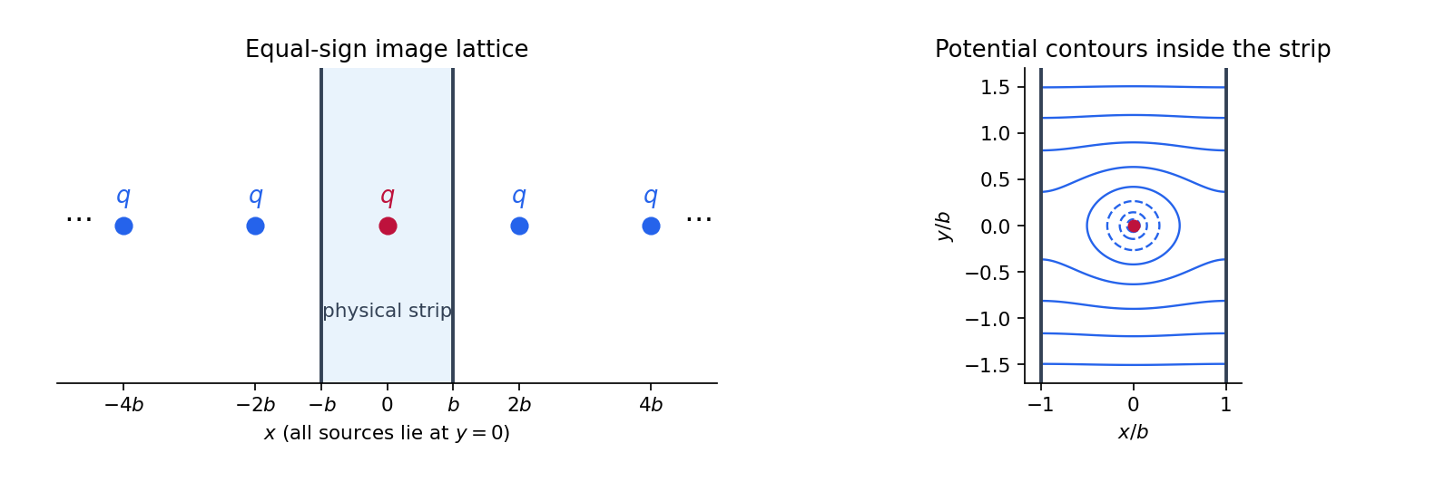
For the two insulating walls, successive Euclidean reflections in and generate sources of strength at for every integer . Only lies inside the physical strip. This is the Neumann image lattice for a point source in a strip. SetThe raw sum of logarithmic potentials diverges by additive constants. A well-defined potential is obtained by pairing opposite images and subtracting their constant reference terms:Each paired summand is on compact subsets away from the source. The series therefore has local uniform convergence, as do the required derivative series. It givesIn the corresponding -derivative, the images pair as and at , and as and at . Their opposite horizontal separations make the derivatives cancel. Thus both homogeneous Neumann boundary conditions hold. The constructed solution is even in ; without a condition at infinity the side conditions alone would allow further homogeneous harmonic functions.
For fixed , uniform convergence on permits integration term by term. The th term has integralHere is the ordinary real inverse trigonometric function, taking values in . Summing from to makes a telescoping series:The source flux splits equally between the upper and lower parts of the strip. The next two parts give the single-wall constructions that underlie the image lattice.


The Dirichlet uniqueness for the Poisson equation follows from a positive integral. Suppose satisfy the same data, and put . Then is a harmonic function in and vanishes on . Green's first identity, applied with both arguments , givesThus , and is constant on the connected body. Its zero boundary value makes that constant zero. This proves at most one temperature field; it does not require an independent existence construction. As usual, the argument assumes a bounded body and sufficient regularity for Green's first identity, or the corresponding finite-energy weak formulation.
For the composite body, let and be the differences in and . They are harmonic functions, have a common interface value , and obeyThe unit normal vector points out of ; the outward normal of on its inner boundary is . Keeping that sign in Green's first identity givesThe outer boundary term in is zero. Weight these equations by the positive coefficients that match the flux condition:Both Dirichlet energies must vanish. Hence both differences are constants; the outer data set the constant in to zero, and interface continuity sets the constant in to zero. This establishes uniqueness for a harmonic transmission problem. Physically and play the roles of the inner and outer thermal conductivities; continuity of temperature and normal heat flux is what cancels the interface contribution.
For the matrices, put , and . Since , and , direct matrix multiplication givesThese verify the listed matrices and the defining relations, with . To check every product explicitly through a single calculation, write elements in the unique form , with and . The relations giveThe displayed matrices obey , so their product has exactly the same form:All exponents are reduced modulo two or three respectively. Thus this verifies all 36 products, and is a two-dimensional complex group representation. It is given to be an irreducible representation.
For a one-dimensional complex group representation , let and , which are nonzero complex numbers. The relations requireSince scalar multiplication commutes and , the last relation gives , hence . Then . The choice is the trivial representation; the unique nontrivial choice is the sign representation:Its group kernel isA faithful representation is injective and has trivial kernel. Here the kernel has three elements, so is not faithful.
Both one-dimensional representations are irreducible representations, and they are inequivalent to each other and to the given two-dimensional one. The sum of squares of irreducible representation dimensions givesThese exhaust all complex irreducible representations. Their number equals the number of conjugacy classes, so there are three conjugacy classes. Explicitly they areThe last two sets consist of the 3-cycles and transpositions respectively.
There are unlisted articles, also show them or only show them.