
Past exam of the physics A course of the University of Cambridge 2017 Paper 2 Section A 5 Solution Created 2026-10-18 Updated 2026-10-20
For fixed electron number , the specified electron degeneracy pressure scales as . Differentiating at fixed low temperature gives the degeneracy-pressure bulk modulus,A monovalent sample has one conduction electron per atom. Its carrier density isusing the Avogadro constant . Substitution with reduced Planck constant and electron mass givesEquivalently, and for this free electron model. This is the assumed electronic contribution, not a calculation of the complete equation of state of real potassium: ionic cohesion and interaction corrections have been excluded as instructed. The supplied pressure is the zero-temperature form, appropriate to leading order for .
Past exam of the physics A course of the University of Cambridge 2017 Paper 2 Section A 4 Solution 2026-10-18
In a conventional face-centered cubic lattice cell of side , touching nearest-neighbour hard spheres lie along a face diagonal. Four radii span that diagonal, so and . In a conventional body-centered cubic lattice cell, the contact lies on the body diagonal: , giving . ThereforeThese are the nonprimitive cubic unit cells requested. They contain four and two atoms respectively, so their volume ratio should not be confused with the volume-per-atom ratio, which is half as large, . The common sphere radius cancels.
Past exam of the physics A course of the University of Cambridge 2017 Paper 2 Section A 3 Solution 2026-10-18
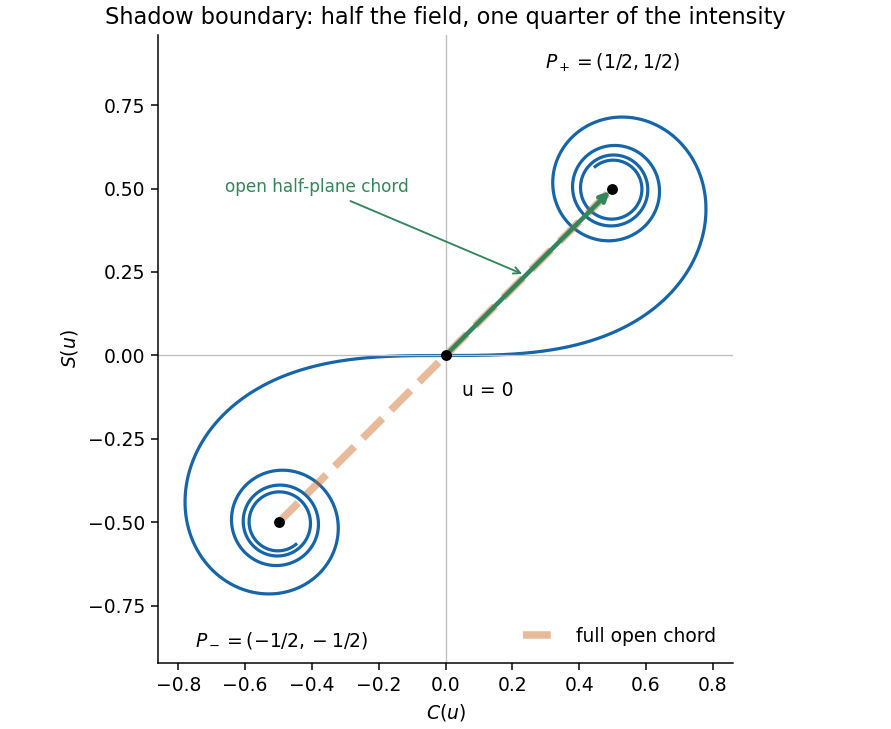
The original diagram puts the upper edge of the obstruction exactly on the straight line from source to detector. The detector is therefore at the geometric shadow boundary, not deep inside the shadow. In the optical convention, the Cornu spiral iswith limiting points and . The unobstructed Fresnel diffraction amplitude is the chord joining both endpoints, proportional to . The open half-plane supplies only the chord from to , proportional to . The coordinate perpendicular to the page contributes the same factor in both cases.This is the half-plane shadow-boundary intensity. The missing half of the aperture removes half the field here, so taking half the intensity would be incorrect.
Past exam of the physics A course of the University of Cambridge 2017 Paper 2 Section A 2 Solution 2026-10-18
For an object near the front focal plane, the objective's numerical aperture in air isThe Rayleigh criterion for a circular objective gives object-space diffraction-limited resolutionThe factor comes from the first zero of the Airy disk. Using the exact changes the result by less than . A coarser estimate gives ; the chosen criterion must be stated. This estimates the aperture limit, before aberrations and detector sampling.
Past exam of the physics A course of the University of Cambridge 2017 Paper 2 Section A 1 Solution 2026-10-18
The characteristic impedance of a stretched string is , since its wave speed obeys . Put the endpoint at and use displacement complex amplitudes incident and reflected:At the massless end, the string's transverse force balances the damper's force . Thus , or . This viscous termination of a stretched string hasHalf the incident mean power is reflected when , giving two positive solutions:They are approximately and , in . The smaller coefficient produces no reflected displacement-phase reversal; the larger produces a reversal. Both dissipate the remaining half of the incident power. Choosing the impedance-matched value would instead absorb all of it.
Past exam of the physics A course of the University of Cambridge 2017 Paper 1 Section D D12 Solution 2026-10-18
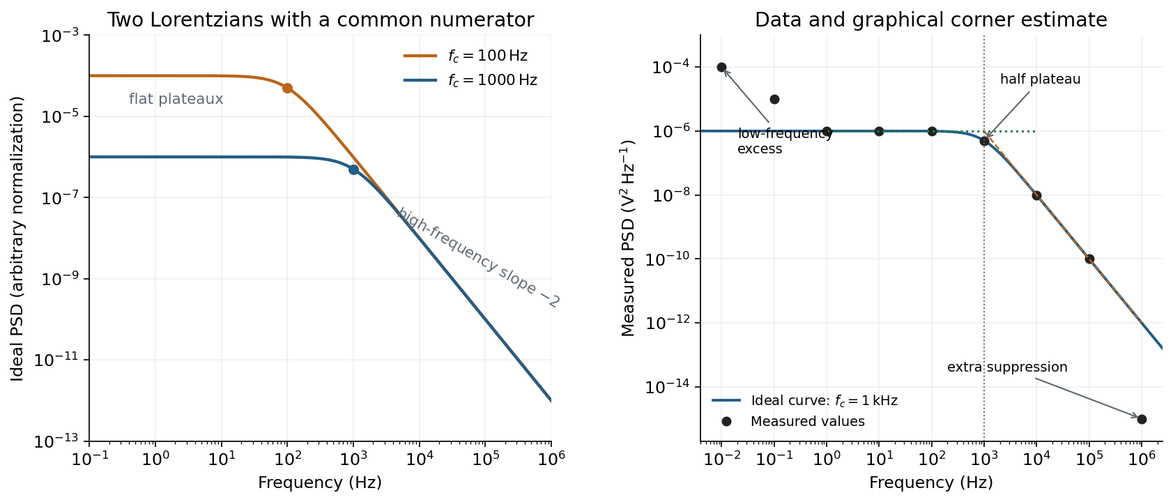
Ideal spectrum. Write , with . The overdamped harmonic-trap power spectrum is a Lorentzian line shape:Thus its log-log plot is horizontal at low frequency and approaches slope at high frequency, changing around . The left panel below compares two characteristic frequencies with the same illustrative ; a common numerator is explicitly assumed for this sketch. Their high-frequency tails coincide and their low-frequency plateaux differ as .
Ideal Lorentzian spectra at two corner frequencies and the measured spectrum with its graphical corner estimate
. Details. The right panel plots all nine original data points, including the very-low-frequency excess and the highest-frequency suppression. It also shows the ideal curve inferred only from the requested intermediate range.
Graphical corner estimate. Between roughly and the measured power spectral density is approximately the plateau . At and ,so the descending asymptote is with . The graphical corner frequency of a Lorentzian spectrum is where these asymptotes intersect:Independently, the measured value is exactly the half-plateau condition . Both graphical readings agree. The inferred ideal curve is approximately
Low-frequency excess and recording duration. The two lowest-frequency measurements increase approximately as , whereas the ideal trapped oscillator tends to a constant plateau. This resembles flicker noise or slow apparatus drift superposed on the motion. The transimpedance amplifier, detector or environment could contribute; the spectrum alone does not identify the source uniquely. It would be incorrect to attribute that whole excess to the ideal Brownian oscillator.
A finite record of duration has ordinary Fourier frequency resolution of order . Resolving the lowest tabulated frequency therefore requires at leastThis is a formal lower bound corresponding to about one cycle; a reliable noise-spectrum estimate normally needs a substantially longer record and averaging.
Sampling. The largest reported frequency is . The Nyquist–Shannon sampling theorem therefore gives the Nyquist lower boundIn practice choose a rate above , with an analogue anti-aliasing filter suppressing unmeasured content above half the sampling rate. Exact equality cannot recover an arbitrary pure sinusoid precisely at the boundary for every phase; it is the limiting lower-bound answer rather than a comfortable practical sampling design.
High-frequency departure and amplifier design. Extrapolating the fitted tail to predicts approximately , while the measured value is . The observed drop from to has effective logarithmic slope , much steeper than the ideal .
A detector or amplifier bandwidth limit, or intentional filtering before digitization, can explain such suppression. For a linear filter the spectral density transformation under a linear filter is , so the last point corresponds approximately to an additional relative voltage gain , if attributed entirely to the readout transfer function. One additional point does not determine a unique filter order or identify the circuit responsible.
Rolling off an amplifier's gain beyond the useful signal band reduces integrated high-frequency noise, suppresses interference, and helps prevent aliasing in the analogue-to-digital converter. Limiting high-frequency loop gain can also improve feedback stability and suppress unwanted oscillation. The cutoff must retain the frequencies needed for the measurement; excessive filtering would distort the desired fluctuation spectrum itself.
Past exam of the physics A course of the University of Cambridge 2017 Paper 1 Section C C10 Solution Created 2026-10-18 Updated 2026-10-20
Operators, quantization and rotations. Angular momentum is the generator of spatial rotations. In quantum mechanics, its components are Hermitian operators on their appropriate domains and obeyThese angular momentum commutation relations prevent all three components from having simultaneous sharp values. For example, the Robertson uncertainty principle gives . One conventionally diagonalizes and a selected component :The allowed labels are and . An angular-momentum multiplet has states. The magnitude differs from the largest possible component ; the remaining components fluctuate even in a state with maximal .
The angular momentum lowering operator and its raising counterpart, , satisfyThe ladder terminates at . A rotation through angle about unit vector acts through the unitary operator . Thus quantized components and the continuous rotation of a state are compatible.
Orbital angular momentum. The orbital contribution is associated with motion in space:For a spinless spatial wavefunction, the simultaneous angular eigenfunctions are the spherical harmonics , with and . Single-valued ordinary scalar spatial wavefunctions give integer orbital labels. In a central potential energy, , so stationary states may be labelled by these angular quantum numbers. The angular kinetic contribution appears in the radial equation as , the centrifugal potential. Noncentral interactions need not conserve these orbital labels.
Intrinsic spin and addition. Spin angular momentum is an intrinsic internal degree of freedom with the same commutation algebra. It is not the angular momentum of a small classical charged sphere literally rotating about its centre. For an electron, and , so in terms of the Pauli matrices. Its squared spin is . Other particles can have integer or half-integer spin, including spin zero.
For one particle with orbital and spin degrees of freedom, ; the two component sets commute with each other. Addition of angular momentum permits . The coupled states are linear combinations of the uncoupled with , determined by Clebsch-Gordan coefficients. A rotationally invariant spin-orbit interaction can conserve while mixing the separate component labels.
Angular momentum also carries a magnetic moment. For an electron's orbital motion and intrinsic spin,The minus signs reflect negative electric charge. With the Bohr magneton , a spin projection has . A magnetic field can therefore distinguish angular-momentum states through their interaction energy .
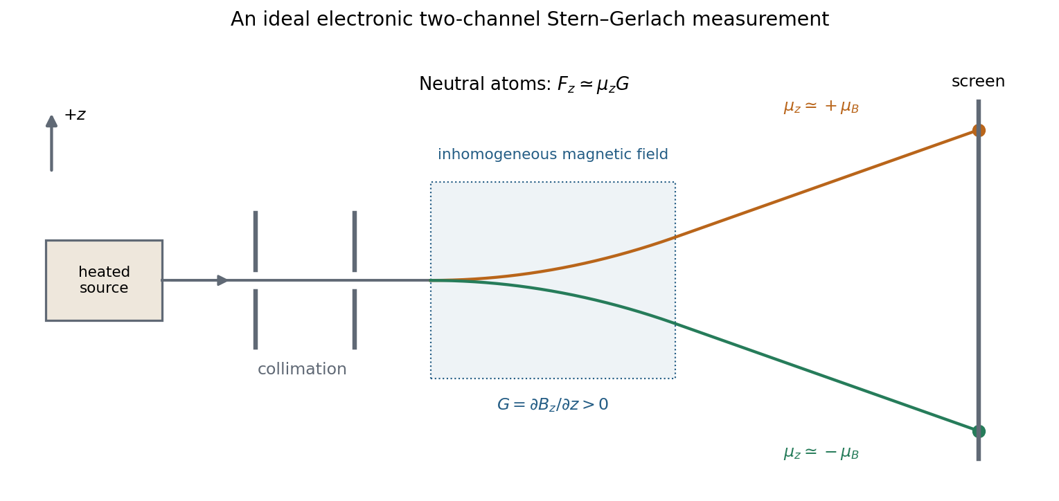
Stern–Gerlach measurement. In the Stern-Gerlach experiment, atoms emerge from a heated source, pass through collimating apertures, traverse a strongly inhomogeneous magnetic field, and strike a position-sensitive screen. The beam is neutral, so its separation is interpreted through the atomic magnetic moment rather than the ordinary charged-particle Lorentz force. Near a chosen quantization direction, the interaction givesA uniform field can exert a torque but would not separate the beam by this translational force; the gradient is essential. Different allowed magnetic-moment components become correlated with different trajectories. A classical ensemble with continuously varying orientations would yield a continuous spread, whereas discrete quantum components yield separated channels.
In the modern electronic description of ground-state silver, filled shells cancel their electronic angular momenta and the unpaired electron has , , . The effective electronic measurement therefore has two components, approximately , rather than an orbital , which is not allowed. For positive field gradient the electronic component has negative and deflects downward in this coordinate convention. Nuclear spin and hyperfine structure are neglected in this simplified two-channel account. Historically the original splitting preceded the electron-spin interpretation, so the modern explanation should not be confused with the original investigators' interpretation.


More generally a prepared spin state gives the two outcomes with probabilities . Selecting one channel prepares a state for further measurements. An ideal second analyser along the same axis then gives a definite result, whereas one along a perpendicular axis gives two equally likely outcomes for a spin-one-half eigenstate. This connects the apparatus directly to incompatible spin components and the Born rule. Angular momentum is quantized through its operator algebra; the Stern–Gerlach gradient turns that discrete internal information into spatially distinguishable outcomes.
Past exam of the physics A course of the University of Cambridge 2017 Paper 1 Section B B9 Solution 2026-10-18
Distinguishable noninteracting particles. Interpret as the same external one-particle potential for each particle; the total potential is . The Time-dependent Schrödinger equation isLet and , where . Applying to the product multiplies it by . The time derivative of multiplies it by . Thus the proposed stationary product is a solution providedThe tensor product separates the two independent one-particle dynamics.
Identical spin-one-half particles. Identical fermions require antisymmetry under exchange of the complete position-and-spin labels. First take to be distinct orthonormal spatial orbitals, and defineThe symmetric spatial state must multiply the antisymmetric spin-one-half singlet state; the antisymmetric spatial state must multiply one of the three symmetric spin-one-half triplet states. The four normalized possibilities, each with the common time factor , areThese are the required product states under fermionic exchange symmetry. If , the antisymmetric spatial combination vanishes. Only the product times the singlet remains, as required by the Pauli exclusion principle. A nonorthogonal pair would require different normalization factors; the displayed assumes an orthonormal stationary-state basis.
Weak repulsive Coulomb interaction. For fixed orbitals , first-order perturbation theory gives spatial energy shifts . Here is the direct interaction energy, while the exchange integral for repulsion strength isThe positivity follows from the positive Fourier transform of the Coulomb kernel. Consequently Coulomb exchange splitting of two orbitals givesAll three triplet spin components remain degenerate for a spin-independent Coulomb interaction. Their antisymmetric spatial factor vanishes at coincidence and reduces close encounters. The inequality is strict when ; for negligible orbital overlap, the splitting may vanish. This comparison fixes one particle in each of the specified orbitals and does not rank singlets with a different orbital occupation.
Spin-zero bosons. For one particle in each of the same distinct orthonormal orbitals, the spin factor is symmetric and bosonic exchange symmetry requires . At coincident positions,Thus the bosonic coincidence enhancement in two orthogonal orbitals isThese are joint probability densities, or small-detector-volume limits; an exactly specified point has zero probability in a continuous distribution. If both particles occupy the same orbital, the properly normalized product is already symmetric and the corresponding enhancement relative to distinguishable particles in that same orbital is one. The paper's usual factor-two answer presumes distinct orthogonal input orbitals.
There are unlisted articles, also show them or only show them.