
Past exam of the physics A course of the University of Cambridge 2017 Paper 1 Section B B8 Solution Created 2026-10-18 Updated 2026-10-20
Reduced radial equation. A spherical harmonic satisfies . Substitute into the time-independent Schrödinger equation, divide out the angular function, and put . Direct differentiation givesMultiplication by then gives the Radial Schrodinger equationHere is the reduced mass, and the extra positive term is the centrifugal potential.
Boundary conditions. At the origin this finite central potential has no point interaction. The physical radial solution is regular there, requiring ; for , a nonzero constant would give and a point-source singularity of the three-dimensional Laplacian. Mere square integrability alone would not remove that singular solution. For a bound state, the radial probability integral is , so the exterior solution must decay and as .
Solutions for zero orbital angular momentum. For and , defineThe interior equation is ; excludes the cosine. The exterior equation is ; normalizability excludes the growing exponential. ThusThe constants cannot remain independent once the interface is matched. Since the potential step is finite, both and are continuous at :Dividing the equations yields
Existence and number of s-wave bound states. Put , , and . ThenThe lowest branch lies on . Along it, and increases continuously from to infinity. Therefore a first negative-energy solution exists precisely when , orFurther branches begin at as . Hence the bound-state thresholds of a spherical square well give exactly one negative-energy state whenThe upper equality is included: the second branch is then only at , with constant exterior , and is not normalizable. If threshold cases are excluded by convention, the commonly quoted open interval has a strict upper inequality; the physical negative-energy state count at equality is still one.
Deuteron estimate. Using , and gives . At ,The threshold for a second state is , far above the stipulated depth . Thus this model has no radially excited s-wave bound state.
Checking other orbital angular momentum sectors matters before ruling out every excitation. At the first -wave threshold, the regular interior reduced radial function is and the zero-energy exterior function is proportional to . Matching their logarithmic derivatives requires , whose first root is . HenceLarger only increases the centrifugal potential. Therefore no bound orbital excited states are expected in the specified central square-well model. Its spin dependence and tensor nuclear forces have not been specified; the calculation does not resolve the real deuteron's internal spin structure.
Past exam of the physics A course of the University of Cambridge 2017 Paper 1 Section B B7 Solution 2026-10-18
Hamiltonian and commutators. Use the canonical commutation relation and define . Expanding the product of the given creation and annihilation operators,Therefore the quantum harmonic oscillator Hamiltonian operator isSimilarly,Using gives
Lowering a normalized energy eigenstate. The commutator impliesFor , nondegeneracy of this one-dimensional energy level means . Its norm is fixed by the number operator:Choosing successive eigenstate phases in the conventional way makes , soFor , the same norm is zero, hence . A nonzero lowered ground state would have energy below the lowest allowed level, and positivity of forbids that possibility.
Coherent-state eigenvalue. Applying the annihilation operator term by term, with the contribution zero, givesThusThe coherent state is normalized because . Its annihilation operator is not Hermitian, so the eigenvalue may be complex.
Time evolution. Under the time-independent Hamiltonian operator, each energy component acquires its own phase:Since , the normalization prefactor is unchanged. HenceThe state remains a coherent state, with its complex parameter rotating at the oscillator's angular frequency; the displayed extra factor is a global phase from the zero-point energy.
Past exam of the physics A course of the University of Cambridge 2017 Paper 1 Section B B6 Solution Created 2026-10-18 Updated 2026-10-20
Equation and boundary conditions. The delta potential has strength with units of energy times length, because the Dirac delta function has units of inverse length. The time-independent Schrödinger equation isThe wavefunction is continuous at the origin. A finite jump in would produce a derivative of a Dirac delta function in , with no corresponding term in this potential. A jump in does produce a delta contribution and is allowed. Integrate through a symmetric interval:For continuous finite , the right-hand side vanishes as . ConsequentlyThis derivative jump is the boundary condition associated with the attractive delta potential.
Unique bound state. For , write . Away from the origin, . Normalizability excludes exponentials growing at either infinity, leavingContinuity gives . The derivative jump then becomes . For a nonzero state,There is exactly one positive value of , so exactly one negative-energy bound state. An odd solution would have ; the allowed decaying exponentials would then both vanish identically. Normalize the even solution usingChoosing the overall phase real and positive gives the bound state in a delta potential:It peaks at the origin, has a downward cusp there, and decays exponentially on both sides. Its value, but not its slope, is continuous.
Scattering amplitudes and fluxes. For , put and retain as a strength parameter. A unit-amplitude wave incident from the left hasContinuity gives . The jump condition givesSolving,The probability current of a plane wave of amplitude is in its propagation direction. Since the asymptotic wavenumber is the same on both sides, reflection probability and transmission probability are just and :They satisfy , expressing conserved probability current in this real potential.
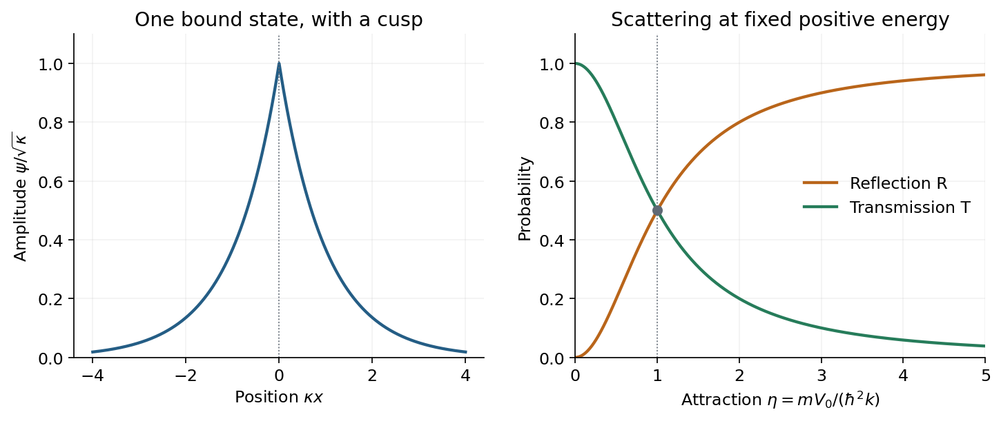
The normalized delta-well bound state and reflection/transmission probabilities as attraction increases
. Details. The right-hand plot uses , proportional to at fixed incident energy. Then rises monotonically from zero to one, while falls from one to zero; they are equal at . Despite the absence of a classical forbidden barrier, an abrupt attractive interaction reflects a quantum wave. Increasing attraction strengthens the derivative mismatch and can approach complete reflection at fixed positive energy. At fixed , increasing incident energy instead makes the well increasingly transparent. The negative-energy bound state and the positive-energy scattering states are different stationary solutions, not an absorptive loss channel.
Past exam of the physics A course of the University of Cambridge 2017 Paper 1 Section A 5 Solution 2026-10-18
Use the sample mean to estimate each magnetic susceptibility, and the unbiased sample variance with denominator to estimate the repeatability of individual readings. In the numerical scale supplied by the paper,If the repeated measurements have independent random errors, their mean estimates have standard errorsThe difference and its estimated standard uncertainty are thereforeThe separation is about standard errors. Under an approximately normal distribution model with no experimenter-dependent bias, Welch's t-test gives about statistical degrees of freedom and a two-sided p-value of . Thus there is modest evidence against equal underlying susceptibilities at a conventional significance level; overlap of the ranges of individual readings is not an adequate comparison of the means. Five readings per sample provide limited information about the error distribution.
Crucially, material and student exhibit complete confounding: each student measured only one sample. An experimenter-dependent systematic error could mimic the difference. Paramagnetism also depends on conditions such as temperature, so equal material alone does not guarantee equal readings without controlling those conditions. The defensible physical conclusion is the data suggest a difference, but do not establish different materials. Both students should measure both samples in randomized or alternating order, with calibration and temperature controlled, to separate a sample effect from an operator effect. No unit or scale factor absent from the original table has been invented.
Past exam of the physics A course of the University of Cambridge 2017 Paper 1 Section A 4 Solution 2026-10-18
Use an inverting operational amplifier. Ground the non-inverting input, connect the source to the inverting input through , and connect from the output back to that same input.
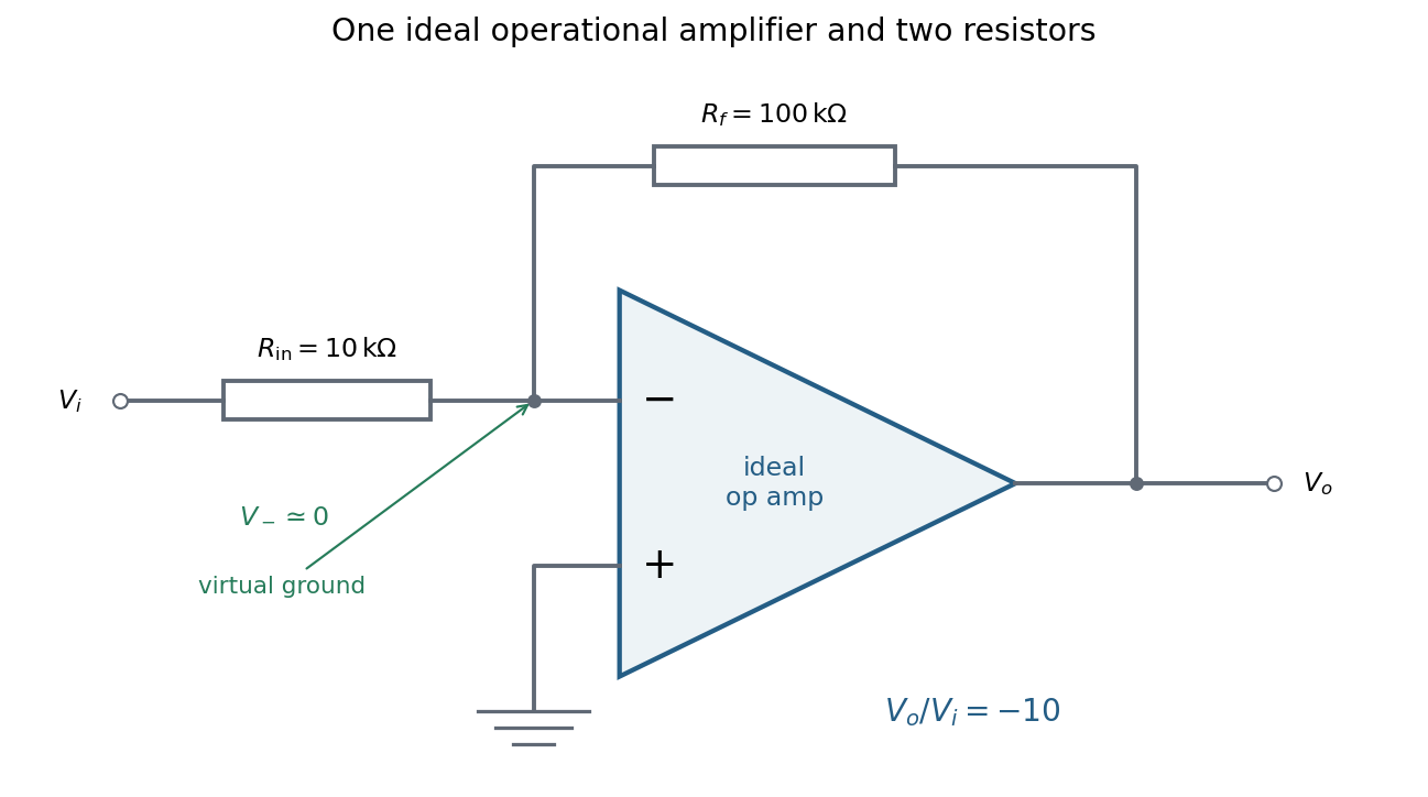
In linear operation the ideal operational amplifier draws no input electric current, and feedback holds the inverting input at the same electric potential as the grounded non-inverting input. This node is a virtual ground. Kirchhoff's current law there givesThe source supplies current , so its input impedance is . The required design is thereforeOnly these two resistors and the single ideal operational amplifier are needed in the signal circuit; its power supplies are implicit. The result assumes an input small enough to keep the output within its linear operating range.
Past exam of the physics A course of the University of Cambridge 2017 Paper 1 Section A 3 Solution 2026-10-18
For addition of angular momentum, the allowed total quantum number runs in unit steps from to . With and ,Thus the complete list of multiplets isThe total angular momentum operator has squared magnitude eigenvalue and chosen-axis component eigenvalue . The number of states is , matching the uncoupled dimension .
Past exam of the physics A course of the University of Cambridge 2017 Paper 1 Section A 2 Solution 2026-10-18
Use the canonical commutation relation on a common invariant domain of the operator products. Write , so . Associativity then giveswhereasThereforeAs a direct position-representation check, the momentum operator is . Acting on a smooth function givesThis is the equality of two quadratic position-momentum orderings; it does not make arbitrary rearrangements of noncommuting linear operators interchangeable.
Past exam of the physics A course of the University of Cambridge 2017 Paper 1 Section A 1 Solution Created 2026-10-18 Updated 2026-10-20
The original diagram places hard walls at and , and the central plateau on is exactly at the indicated ground-state energy. This equality determines the middle of the requested sketch. In the time-independent Schrödinger equation,the central interval has , hence . The ground state can be chosen real and positive inside the walls by the nodeless theorem for a one-dimensional ground state. Reflection symmetry makes it even about , so its linear central segment must be constant.
The hard-wall boundary conditions are . On both outer intervals , so the positive wavefunction has negative curvature and is sinusoidal. Wavefunction matching at a finite potential step requires both and to remain continuous at ; the derivative therefore vanishes where each sinusoidal flank meets the flat middle. A normalized representative isEach side contributes and the plateau contributes to the squared norm before multiplying by . The corresponding consistency condition is ; a numerical energy is not required for the sketch.
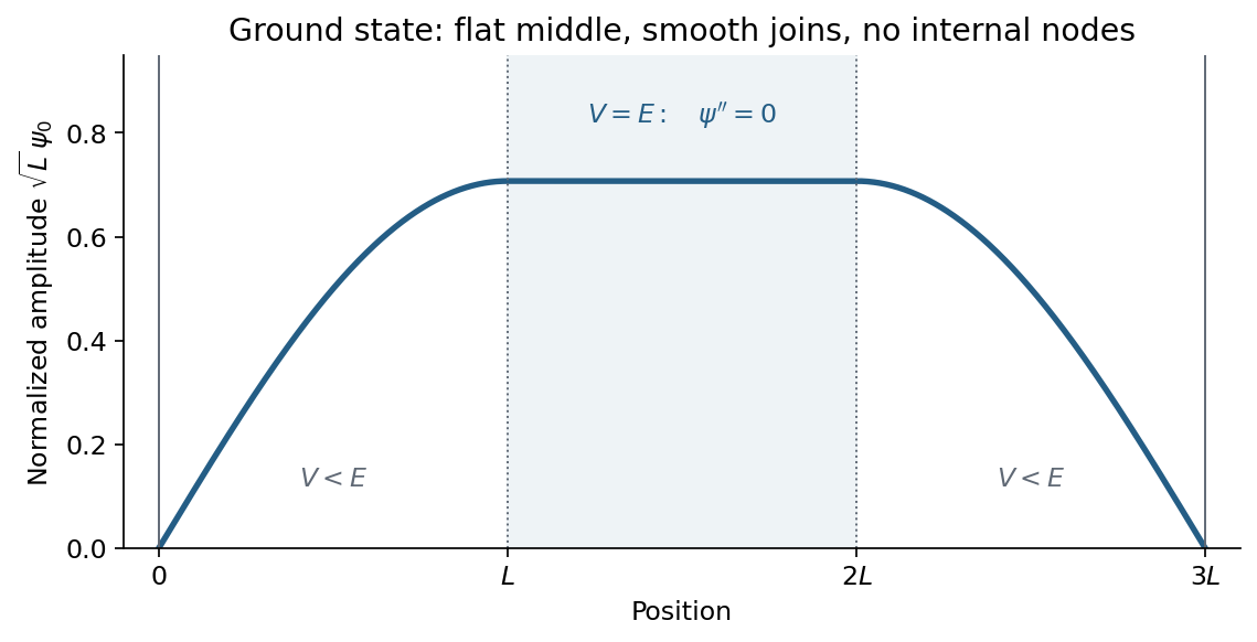
The positive ground-state wavefunction has sinusoidal flanks and a flat central segment at V equals E
. Details. Thus the ground state at the top of a central rectangular barrier has no internal nodes, continuous value and slope, and a flat middle, rather than an exponential dip through a classically forbidden region. Multiplication by an overall constant phase changes none of these physical features.
Past exam of the particle and nuclear physics course of the University of Cambridge 2022 Section B 6 e Solution Created 2026-10-18 Updated 2026-10-20
The table gives the Xi baryon mean lifetime . At , an initially resting particle has survival probabilityThus the most probable contents are one undecayed . The initial momentum is unspecified. For a moving parent, time dilation replaces the denominator by , making the survival probability at least as large. The times below are characteristic proper mean lifetimes; laboratory times depend on the particle velocities.
The principal first step isIt typically occurs on the scale. The neutral pion almost immediately converts to two photons, with and . The Lambda baryon has and two dominant routes.
In the charged-pion route,The muon lifetime is a standard additional input, not present in the supplied five table pages.[ref]
Review of Particle Physics by Particle Data Group (2022). Muon listing, mean-life entry: approximately 2.197 microseconds
The successive contents are approximately , then , then . After a few muon lifetimes the dominant stable endpoint isThe leading-path probability including the tabulated two-photon pion branch isHere the last factor is the tabulated dominant muonic charged-pion fraction; rare radiative corrections are being neglected in describing a fixed photon count. Before selecting pion decay channels, the probability of reaching the history is .In the neutral-pion route,This produces by roughly the nanosecond scale. It is a long-lived intermediate state, not the final endpoint: the free neutron has in the original table and eventually undergoes beta-minus decay,Thus after several thousand seconds the dominant stable endpoint isBefore selecting the two decays, the history has probability . The familiar rough description is therefore a charged-pion route and a neutron route; including the specified leading pion branches gives approximately and for the two displayed endpoints. The remainder includes Dalitz decays and other rare channels, not a failure of probability conservation.
These are particle decay cascades, treating the separated final proton, electron, photons and neutrinos as stable asymptotic particles and neglecting subsequent collisions and rare extra radiation. An infinitely large box prevents escaping particles from being removed from the inventory. Neutrino labels specify their production flavours. Each lifetime describes a stochastic waiting time, so there is no finite sharp instant at which every unstable particle has certainly decayed.
For (i), CP symmetry relates the negative- and positive-pion radiative channels to excellent accuracy. The original positive-pion table therefore predictsThe comparison requires the same photon-energy and event-selection definition. The table attaches an unexplained footnote to this radiative channel; it does not specify those cuts in the supplied excerpt. An arbitrarily soft photon is not a separately infrared-finite exclusive observable, so the numerical value must retain the table's definition.
Part (ii) contains an apparent notation error in the original PDF as well as the TeX: it prints , rather than . Taken literally, the charged leptons carry net electron-family lepton number , and the printed adds another . The initial pion has zero lepton number. This is a channel, not the charge conjugate of the listed positive-pion decay. In the ordinary lepton-number-conserving Standard Model approximation,Allowing lepton-number-violating masses for Majorana neutrinos would require additional physical assumptions and does not justify assigning the tabulated number to that channel.
For the likely intended charge-conjugate process, the prediction is insteadThis distinction follows from a lepton-number test of a decay channel; replacing the printed neutrino by an antineutrino must be stated explicitly.
Both formal processes use one weak charged current transition, with a virtual W boson producing the lepton pair. Two representative lowest-order quark-line diagrams are shown below. They use the component of ; attachment to the antiquark line in the component gives the other contribution to the same hadronic current.
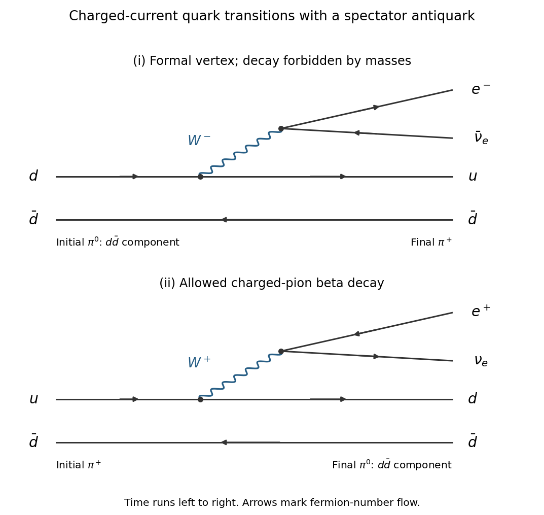


In the first diagram, and , with a spectator quark. In the second, and , again with a spectator . The diagram for the first process describes the coupling but cannot make an energetically forbidden on-shell decay occur.
From the original tables,Therefore the first process has Q valueand is forbidden for an isolated pion. The second hasThe table therefore lists only the second, pion beta decay, withIts tiny branching fraction combines a weak interaction with an exceptionally small available energy. An allowed semileptonic transition has a decay width scaling approximately as , where , with electron-threshold and recoil corrections. The fifth power makes the few-MeV gap especially restrictive. Unlike direct , this semileptonic channel is not forced to have an amplitude proportional to ; its primary extra suppression is the small phase space. Its approximately Cabibbo-favoured current does not supply a further large flavour suppression. The observed branching fraction corresponds to a partial decay rate of about , competing with the much faster dominant muonic decay.
Past exam of the particle and nuclear physics course of the University of Cambridge 2022 Section B 6 b Solution Created 2026-10-18 Updated 2026-10-20
The original table gives the dimensionless branching fractionsThus the four-lepton channel is about times as frequent, despite its smaller available phase space.
The dominant neutral-pion interaction is with two photons. In double Dalitz decay, both are virtual and convert to separate electron-Positron pairs:This requires two electromagnetic conversions but does not force the whole final state into a helicity-suppressed two-fermion configuration. The two virtual photons and four final leptons allow the necessary angular momentum correlations.
For the two-lepton mode, a single virtual photon cannot mediate a pion into : the electromagnetic vector current has the wrong quantum numbers. The leading electromagnetic mechanism involves two virtual photons attached to the same lepton line, with a loop integration. The resulting pseudoscalar two-lepton amplitude vanishes as , so its decay width has an additional helicity suppression factor proportional to .
Both channels involve extra electromagnetic couplings relative to . The crucial distinction is the extra leptonic loop and helicity suppression of the two-lepton channel; counting final particles or couplings alone misses it. The pion-two-photon interaction itself already contains strong-interaction structure, so “extra loop” here compares the diagrams after representing that common interaction by an effective vertex.
The charged pion has spin zero. In its rest frame, the outgoing muon or Positron and the neutrino travel in opposite directions. With a nearly massless left-helicity neutrino, total angular momentum zero requires the positive charged antilepton to have negative helicity. The weak charged current instead creates a massless positive antilepton with positive helicity. A nonzero charged-lepton mass supplies the required opposite-helicity component.
Thus the decay amplitude is proportional to : this is helicity suppression. Explicitly, contracting the pion's axial-current matrix element, proportional to its four-momentum , with the leptonic current and applying the Dirac equation leaves a factor . The leptonic pseudoscalar decay width is, in the convention,The phase space advantage of the lighter Positron cannot offset its much stronger helicity suppression. The common factors cancel in the pion electron-to-muon decay ratio:This tree-level estimate explains why the muonic branch dominates by roughly four orders of magnitude. The paper's table gives an electronic branching fraction ; electromagnetic corrections change the simple ratio by a few percent without changing the mechanism.
The predicted-minus-measured differences areRelative to the measured masses, these are and . The predicted spin-spin interaction splitting is , compared with the measured , a discrepancy of about in the splitting.
This is an effective constituent-quark model, with a common spatial contact factor and a nonrelativistic spin-dependent interaction applied to light quarks. Relativistic motion, different spatial wavefunctions, and omitted strong-interaction corrections prevent an expectation of accuracy at the experimental -- scale. Agreement at the level of several percent in absolute baryon masses would already be useful for such a simple formula; the sub-percent absolute-mass agreement here is better than that rough expectation.
No theoretical uncertainty or fitting prescription is supplied, so there is no unique numerical “expected error” or justified statistical significance to attach to the deviations. Small relative errors in the large spin-independent mass sum also need not imply equally small relative errors in the much smaller spin-spin interaction splitting.
Use GeV consistently with the supplied :The spin-independent sum is . The spin-spin interaction corrections areThusThe displayed decimal places document the calculation, rather than asserting that this simple constituent-quark model has sub-MeV predictive precision.
Label the identical strange quarks as 1 and 2 and the up quark as 3. In the ground spatial state, the pair has symmetric space and flavour factors but an antisymmetric colour factor. The Pauli exclusion principle therefore requires a symmetric spin factor: the pair has .
The angular momentum identitygivesNext couple to , where . For total ,For the spin- Xi baryon, this is . By symmetry the two pair correlations are each . Inserting the pair correlations into the baryon hyperfine mass formula givesFor the spin- state, the same coupling gives . Each pair correlation is therefore , as expected for a fully symmetric spin state. HenceThe predicted splitting is a useful independent check:
Past exam of the particle and nuclear physics course of the University of Cambridge 2022 Section B 5 b Solution Created 2026-10-18 Updated 2026-11-05
The baryon hyperfine mass formula is a phenomenological constituent-quark model. The three constituent quark masses include effects of strong-interaction dressing and an approximate spin-independent confinement energy; they are not the small running quark masses in a short-distance quantum chromodynamics calculation.
The residual correction has the form of a colour-magnetic spin-spin interaction. A nonrelativistic reduction of one-gluon exchange produces a contact contribution proportional toAfter taking its expectation in the common spatial wavefunction and the colour singlet, the colour factor, coupling, and contact density are absorbed into . Summing the three quark pairs gives the supplied formula. Positive raises aligned-spin configurations relative to lower-spin configurations. In natural units, the spin angular momentum operators are dimensionless, so has units of energy cubed, as in the given .
A ground-state baryon contains three quarks in a spatially symmetric wavefunction, giving positive parity. Each quark is a spin one-half fermion, so the complete wavefunction must be antisymmetric under interchange of its complete quark labels. A physical baryon is a colour singlet, with the antisymmetric colour factorConsequently the combined spin-and-flavour factor must be symmetric. The product notation in the question organizes the degrees of freedom; it need not mean that spin and flavour are separately unentangled. In particular the octet requires a correlated sum of products.
For the three light flavours, the flavour symmetry decomposition isThe subscripts describe permutation symmetry, with denoting mixed symmetry. The addition of angular momentum of three spin one-half particles givesThe symmetric spin quartet has total ; the two spin doublets have .
For , the spin factor is symmetric, so the flavour factor must also be symmetric: this gives the spin- baryon decuplet. Its flavour content is four states, three states, two states, and one state.
For , the mixed-symmetry spin functions combine with the mixed-symmetry flavour functions to make one fully symmetric spin-flavour factor for each octet weight: this gives the spin- baryon octet, containing two nucleons, three Sigma baryons, one Lambda baryon, and two Xi baryons. The two mixed-symmetry octets in the raw flavour product are not two distinct ground-state octets; their permutation partners are correlated with the spin factors. An antisymmetric flavour singlet would require a fully antisymmetric spin factor to make a symmetric product, but three spin states drawn from a two-dimensional single-quark spin space have no such factor.
Equivalently, the symmetric three-particle representation of spin-flavour symmetry has dimension and decomposes under flavour and spin intoThese are approximate multiplets: the larger strange quark mass breaks exact flavour symmetry and splits their energies.
There are unlisted articles, also show them or only show them.