
Past exam of the soft condensed matter course of the University of Cambridge 2017 3 a Solution 2026-10-18
Molecular area from the adsorption slope. The supplied Gibbs adsorption equation identifies the surface excess number density throughThe logarithm is understood relative to a fixed concentration unit or reference concentration; only concentration ratios enter its differences. The pure-water point supplies a baseline surface tension, but cannot be included in .
An estimate near the later working concentration uses its two bracketing points:Taking room temperature as ,This corresponds to about adsorbed molecules per . The data are not perfectly linear in , so the inferred molecular area depends somewhat on the concentration range: a fit to all five positive-concentration points gives about , while the higher-concentration region gives roughly . An effective area of order – is justified; a concentration-independent exact value is not.
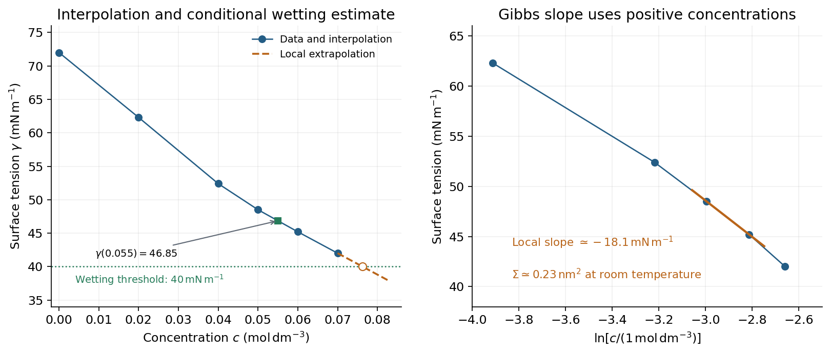
Surface-tension interpolation and extrapolated wetting threshold, alongside the local Gibbs adsorption slope
. Details. 
Contact angle. Linear interpolation between and gives . For an ideal equilibrium contact angle measured through the liquid, Young's equation isThe supplied solid-vapour and solid-liquid values have difference . HenceThis assumes clean homogeneous equilibrium interfaces, negligible contact-angle hysteresis, and the stated solid interfacial energies applicable to the solution.
Complete wetting. The spreading coefficient is . The onset of complete wetting occurs at , or , if the solid interfacial energies remain unchanged. The last measured value is still , so this requires extrapolation beyond the table.
Continuing the last local slope in concentration, per , givesContinuing a constant local Gibbs slope in instead gives approximately . Thus the data suggest a threshold near under continued-trend assumptions, rather than fixing one exactly. A surface-tension plateau caused by micellization, or a change in , could prevent or shift this threshold; no such extra data are given.
Capillary rise. For a circular capillary of radius , vertical surface-tension force balances the weight . Thus capillary action givesUsing , and ,This is the height above the reservoir level in the ideal static capillary approximation; meniscus-volume corrections and contact-angle hysteresis are neglected. The positive gives a rise, rather than a depression.
Past exam of the soft condensed matter course of the University of Cambridge 2017 2 c Solution 2026-10-18
The requested model is the standard linear solid model: a spring of modulus in parallel with a Maxwell branch consisting of a spring in series with a dashpot of viscosity . Both parallel branches have the same strain; their stresses add. In the Maxwell branch the spring and dashpot have the same stress and their strains add. The equilibrium spring prevents indefinite flow at long times.
For harmonic strain , define the dynamic modulus by . The Maxwell branch has compliance . Defining therefore givesThe same mechanical model can represent a shear modulus if the appropriate shear stresses and strains are used consistently.
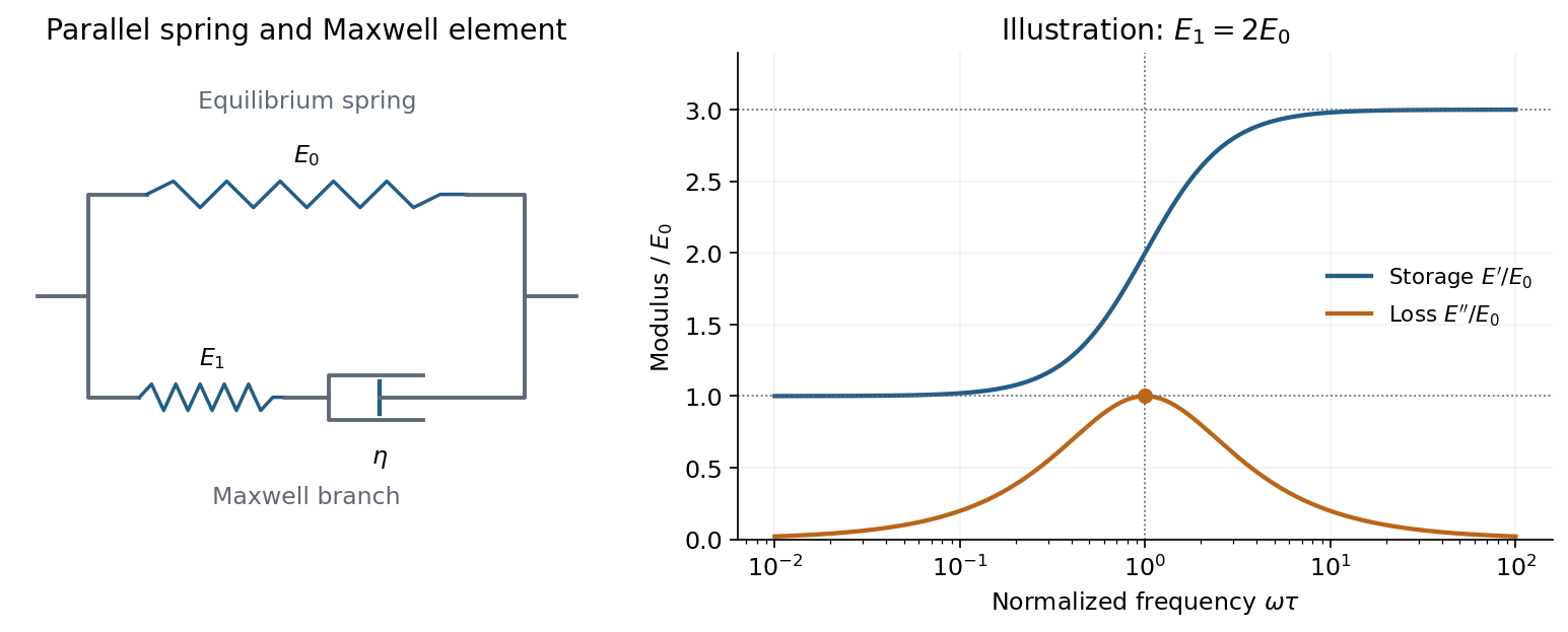
A spring parallel to a Maxwell element gives finite low- and high-frequency storage moduli and one loss-modulus peak
. Details. 
Writing , its storage modulus and loss modulus areWith this time convention the physical stress is and leads the strain by the loss angle. The dissipated energy per unit volume per cycle is . Thus describes elastic storage and describes dissipation.
At low frequency, , the dashpot flows during a cycle and relaxes the Maxwell spring, leaving , . At high frequency, , the dashpot hardly deforms within a cycle, so both springs carry elastic load: , while . The loss modulus is maximal at , with peak value .
The equivalent constitutive equation isAfter a sudden strain is imposed and held, the stress relaxes as . It falls from the instantaneous modulus to the nonzero relaxed modulus . This single-time relaxation is the simplest improvement over a purely elastic solid or a Maxwell fluid with zero long-time modulus.
The loss tangent is . Its maximum need not coincide with the loss-modulus maximum: the peak frequencies in a standard linear solid give for the loss tangent. The model captures one viscoelastic crossover between two finite elastic plateaux, with dissipation concentrated near the relaxation frequency.
Past exam of the soft condensed matter course of the University of Cambridge 2017 2 b Solution 2026-10-18
A grafted polymer chain is tethered to a surface at one end. Let its isolated coil size be , where is the number of statistical units and their statistical segment length. For a good solvent, the Flory approximation gives ; an ideal chain has . Let be the number of tethers per unit area, distinct from the membrane tension in Question 1. Their typical lateral separation is .
At low coverage, , the chains hardly overlap. Each forms a polymer mushroom, retaining roughly the isolated-coil conformation apart from the constraint of the solid surface. Raising coverage until makes neighboring coils overlap. The crossover criterion isFor in a good solvent, maintaining isolated coil shapes would crowd segments into the same lateral regions, increasing excluded-volume and osmotic free energy. Chains stretch predominantly away from the surface to relieve that crowding, at the cost of their conformational entropy. The resulting dense tethered layer is a polymer brush.
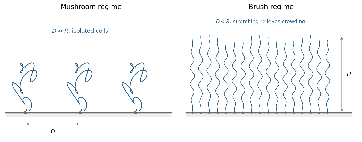
Sparse grafted coils form mushrooms; overlap at higher grafting density stretches chains into a brush
. Details. 
A simple scaling estimate makes the balance explicit. For brush height , the monomer concentration is of order . The free energy per chain in units of iswhere is the effective segment excluded volume. The first term is Gaussian stretching; the second is the cost of segment crowding in a good solvent. Minimizing with respect to height givesWhen , this is . Height increases with chain length and grafting density, while the lateral spacing is fixed by the attachment points. The estimate assumes stretching strong compared with an isolated coil but still much smaller than contour length ; it does not describe fully extended chains. Poor-solvent attraction can instead collapse the layer, so solvent quality must be specified before using the good-solvent formula.
The mushroom-to-brush change is a crowding crossover for finite chains, rather than automatically a sharp thermodynamic phase transition. A swollen brush can provide steric stabilization: bringing two coated surfaces together further compresses and crowds their chains, producing a repulsive free-energy cost. The controlling comparison is tether separation versus isolated coil size, and the brush height follows from competition between chain stretching and segment interactions.
Past exam of the soft condensed matter course of the University of Cambridge 2017 2 a Solution 2026-10-18
The Reynolds number compares inertial and viscous terms in the momentum equation:Here is fluid mass density, a characteristic speed, a swimmer or flow length, and the dynamic viscosity. The advective inertia scale is and the viscous force-density scale is , whose ratio is Re. For an illustrative micron-scale swimmer with and in water, taking and gives .
At such low Re, Stokes flow is the useful approximation. For an incompressible Newtonian fluid it obeys and , with negligible inertia. Swimming is not a sequence of propulsive impulses followed by coasting: drag balances propulsive forces almost instantaneously. For example, the drag on a slowly translating sphere is . A freely swimming organism has approximately zero total external force and torque; its body motion balances the forces and torques generated by its appendages.
The linear equations have kinematic reversibility of Stokes flow: reversing the boundary velocities reverses the fluid motion. A reciprocal stroke that retraces exactly the same sequence of shapes therefore retraces its displacement. This is the scallop theorem. A single hinge opening and closing along the same shape path cannot propel an ideal swimmer through an otherwise quiescent Newtonian Stokes fluid, regardless of merely changing how quickly it opens relative to closing.
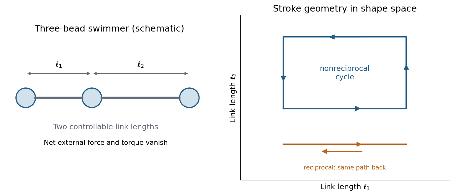
A three-bead swimmer can use a nonreciprocal loop in its two-length shape space, unlike a retraced one-parameter stroke
. Details. 
A useful design has at least two shape coordinates driven out of phase, so the stroke follows a loop rather than a retraced line in shape space. In the three-bead example the two link lengths change in a cycle; hydrodynamic interactions differ at different points of the cycle, allowing net translation. The drawing illustrates this mechanism without assigning a particular swimming speed.
Biological routes include continuous rotation of a chiral helical flagellum, nonreciprocal ciliary strokes, and traveling bending waves along a flagellum. An elongated filament generally has greater drag for motion normal to itself than along itself; this drag anisotropy helps convert those motions into propulsion. The body may counterrotate to balance appendage torque. Micro-organisms must exploit nonreciprocal shape changes, rotation or another mechanism consistent with viscous force balance; inertia-based swimming intuition fails. Viscoelastic surroundings or appreciable inertia can invalidate the particular Newtonian assumptions behind the simple scallop result.
Past exam of the soft condensed matter course of the University of Cambridge 2017 1 c Solution 2026-10-18
Write the membrane height above its mean plane as a sum of Fourier modes, . The supplied average is a thermal mean-squared modal height; for complex Fourier coefficients it is understood as , with for a real height field. The terms are:
- is the thermal energy, with Boltzmann constant and absolute temperature .
- is the projected membrane area used in the Fourier normalization.
- is the in-plane wavenumber; the corresponding wavelength is .
- is the membrane tension, in .
- is the membrane bending modulus, in joules.
In the small-slope approximation, Helfrich membrane energy containsThe equipartition theorem, with the independent real modes counted consistently, gives the stated membrane fluctuation spectrum under tension. Its units are length squared: and both have units , so has units .
At small length scales, is large and the bending term dominates:The fluctuation amplitude is controlled mainly by the membrane bending modulus and thermal energy, rather than tension. The crossover occurs when , henceThe bending-dominated regime extends up to the membrane elastic length when scale means , or up to when it means wavelength. At still larger scales tension gives a spectrum. At the opposite end, the continuum formula requires wavelengths larger than the microscopic membrane thickness or molecular cutoff. Without numerical and , no numerical crossover scale is determined.
Past exam of the soft condensed matter course of the University of Cambridge 2017 1 b Solution 2026-10-18
For an ideally dissociated electrolyte, the Debye–Hückel screening length isHere is ionic number density, the charge in units of the elementary charge, and is molar concentration. Conversion between and number density cancels in a ratio. At fixed relative permittivity, .
In sodium chloride, , giving . Complete dissociation of aluminium chloride gives and , soThe factor is sixty, not ten: the squared charge and the three counterions per formula unit both matter. Using the given reference length directly, and , ,The modest temperature increase raises the screening length by only about at fixed concentration; the large increase in ionic strength shortens it by almost an order of magnitude overall.
Under charge stabilization of colloids, the electrostatic double-layer repulsion now has a much shorter range. Attractive Van der Waals forces can then dominate at closer separations, reducing the barrier to particle aggregation in DLVO theory. Thus an electrostatically stabilized colloid is likely to be destabilized, with aggregation more likely than in the original dispersion.
This is a conditional physical prediction, not a proof of instability from a length alone. No particle radius, surface potential, attractive interaction strength or steric coating is specified. Steric stabilization could preserve stability, and trivalent-ion adsorption can alter the surface charge. Moreover, ideal screening theory is only an estimate at , where ion association, hydrolysis and activities can matter. The numerical result uses the supplied reference length and the stipulated unchanged permittivity, rather than replacing either with an unprovided calibration.
Past exam of the soft condensed matter course of the University of Cambridge 2017 1 a Solution 2026-10-18
Entropic elasticity. A rubber contains flexible polymer strands tied into a network by cross-links. Stretching biases the strands toward relatively extended configurations, reducing their configurational entropy. The restoring entropic force follows from the increase in Helmholtz free energy . For a Gaussian strand with statistical steps of length , its deformation-dependent free energy is approximately . Its stiffness therefore increases with absolute temperature, even if the underlying bond stiffness changes little.
In the ideal affine-network model of rubber elasticity, the shear modulus iswhere is the number density of elastically active network strands. Thus heating increases the modulus approximately in proportion to , provided the network density and rubbery state remain approximately unchanged. Thermal expansion, changing relaxation times or damage can modify that simple trend.
Examples are lightly crosslinked natural rubber, based on cis-rich polyisoprene, and crosslinked polydimethylsiloxane. The crosslinks prevent the long-time macroscopic flow of an unconnected chain solution.
Density estimate and the unspecified modulus convention. With room temperature , the Boltzmann constant gives . If the stated modulus is , thenThe molar value counts moles of active strands. If “modulus” instead means Young's modulus , a nearly incompressible isotropic rubber has , and the inferred value isThus the robust order-of-magnitude estimate is . The cross-link density inferred from rubber elasticity is usually an effective strand density; the actual junction density is for junction functionality in an ideal network without inactive loops or dangling ends. For four-functional junctions this would be half the strand density. The paper supplies neither modulus type nor junction functionality, so a unique chemical junction count cannot be extracted.
Past exam of the relativity course of the University of Cambridge 2022 Section A 3 Solution 2026-10-18
For a grazing null geodesic, take the impact parameter as . The leading Schwarzschild light deflection isWith the gravitational constant and speed of light ,Here , so the weak-field approximation is appropriate. A ray passing at a larger impact parameter has a correspondingly smaller deflection.
Past exam of the relativity course of the University of Cambridge 2022 Section A 2 Solution 2026-10-18
The metric tensor and its inverse are diagonal: , , , on a patch where . Only is nonzero. The Christoffel symbol formula therefore giveswith all other components zero. Using the stated Riemann curvature tensor convention,so . This is the curvature of a two-dimensional warped metric; its Gaussian curvature is .
There are unlisted articles, also show them or only show them.