
Past exam of the mathematics course of the year 2 of the natural sciences course of the University of Cambridge 2008 Paper 2 4 Solution Created 2026-10-18 Updated 2026-10-20
For a simple pole, the residue is , the coefficient of its Laurent series. On an anticlockwise circle , integration of each Laurent term is zero except , whose integral is . This proves the stated single-pole residue theorem.
For , the only pole inside the rectangle of height is , with residue . The residue theorem therefore gives . The upper edge is traversed from right to left and satisfies , so the two horizontal contributions sum to .
On the right edge the modulus is bounded by , and on the left by . Multiplying by the fixed edge length shows that both contributions tend to zero because . ThusUsing yieldsThis rectangular contour for an exponential beta integral also gives the ordinary beta integral after the substitution .
Past exam of the mathematics course of the year 2 of the natural sciences course of the University of Cambridge 2008 Paper 2 3 Solution Created 2026-10-18 Updated 2026-10-20
Away from its source, a radial two-dimensional Green's function satisfies , so . The divergence theorem on a disk of radius around the source requires , hence and . Choosing the additive constant givesThe equality with the Dirac delta is distributional; away from the source the Laplacian vanishes.
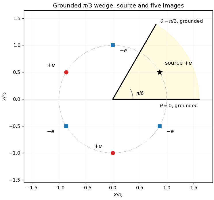
For the wedge, use the finite image construction for a planar wedge. In complex coordinates , place three positive sources at and three negative sources at , . The positive source at is the actual charge. The five images are thereforeOn either grounded ray, reflection pairs each positive source with an equally distant negative source, so their logarithmic potentials cancel. All images lie outside the open physical wedge. Summing their contributions with coefficient gives the required potential. The figure shows the bisecting-source configuration.

Past exam of the mathematics course of the year 2 of the natural sciences course of the University of Cambridge 2008 Paper 2 2 Solution Created 2026-10-18 Updated 2026-10-20
Let be the -periodic ramp represented by on . The Fourier series of a periodic sawtooth givesBoth boundary data are multiples of this odd function, so their angular means and cosine coefficients vanish. Consequently . Put . Matching the sine coefficients at the two radii gives and . Solving this two-by-two linear system yieldsEquivalently, two-boundary annular harmonic interpolation expresses the same solution asEvery term is a harmonic function, and the radial factors enforce the specified boundary values. For a radius strictly between and , their geometric decay makes the series smooth. At the boundary discontinuity , the limiting Fourier value is the mean of the two one-sided values, zero. The boundary data are imposed away from that exceptional point, as stated.
Past exam of the mathematics course of the year 2 of the natural sciences course of the University of Cambridge 2008 Paper 2 10 Solution Created 2026-10-18 Updated 2026-10-20
Let . Since and , its powers define the representation of the cyclic group of order four:For the quaternion group, denote the three displayed complex matrices by . Direct multiplication gives , , , and . Together with the images of , these are exactly the quaternion multiplication relations, proving that the assignment defines a group homomorphism into .
Use the realification of a complex representation: for , define . It acts on grouped real and imaginary coordinates and satisfies . The explicit generators areSet and to specify all eight elements.
For an invertible real , the equivalent representation obeys . The trace is invariant under similarity, so their characters agree. Explicitly,
Past exam of the mathematics course of the year 2 of the natural sciences course of the University of Cambridge 2008 Paper 2 1 Solution Created 2026-10-18 Updated 2026-10-20
Use the weighted inner product with positive weight . For a self-adjoint operator and nonzero eigenfunction , self-adjointness gives . The positive norm therefore forces to be real. For two eigenfunctions of distinct eigenvalues, the same calculation gives , proving their orthogonality.
The Chebyshev differential equation takes the Sturm-Liouville formIts operator is , so as required. For , direct substitution gives . Comparing coefficients yieldsExplicitly, using ,The endpoints are singular because vanishes and diverges there. The polynomial solutions use the natural condition at each end; under these are the Neumann eigenfunctions of the Chebyshev differential operator, proportional to . They differ from the zero-value endpoint realization of the same differential expression.
Past exam of the mathematics course of the year 2 of the natural sciences course of the University of Cambridge 2008 Paper 1 9 Solution Created 2026-10-18 Updated 2026-10-20
Take fixed-endpoint variations with . The first variation isThe boundary term vanishes by the endpoint conditions. The fundamental lemma of the calculus of variations gives the Euler-Lagrange equation . Along its solutions,When , this proves the Beltrami identity .
For the surface , the line element is . The arc-length integrand for a graph is . It has no explicit dependence and satisfies . Thus is constant. Choosing the fixed direction along a smooth nonconstant segment and integrating yieldsThe same result follows by defining the transverse arc coordinate , which changes the metric to . Its geodesics are straight lines in coordinates. This proves the formula for geodesics on a generalized cylinder and shows it gives locally shortest paths. The additional straight lines in the unrolled plane are also geodesics, but cannot be represented as graphs . Classical differential-geometric statements assume the surface has sufficient smoothness; the arc-length coordinate itself only requires the displayed integral to be well defined.
Past exam of the mathematics course of the year 2 of the natural sciences course of the University of Cambridge 2008 Paper 1 8 Solution Created 2026-10-18 Updated 2026-10-20
Termwise differentiation of the convergent Frobenius series and collection of powers in the Bessel differential equation gives the lowest coefficient , the next coefficient , and, for , the coefficient . Since , the stated choices , and the recurrence make all coefficients vanish.
For , the two resulting even-coefficient series areandThese are linearly independent on and give the Bessel functions of order one half, up to normalization. The specified condition is sufficient; in the negative-exponent branch at this particular order the next coefficient equation alone would allow to be free, adding a multiple of the positive-exponent solution.
For the Legendre differential equation, substitution gives the full conditionsThus permits arbitrary , while requires . This Frobenius recurrence for the Legendre equation separates the even and odd series. The nearest singular points of the differential equation are , so the series about zero has radius at least one, and the generic nonterminating solutions have radius exactly one. Particular cancellations can give a larger radius.
Termination occurs when the degree reaches a nonnegative integer with . For this givesChoose the even branch for even or the odd branch for odd to obtain a Legendre polynomial. The recurrence then terminates and gives a solution for all real , with infinite radius of convergence. A nonzero entire solution at other is impossible: each nonterminating parity has coefficient ratio tending to one in the variable , and so radius one.
Past exam of the mathematics course of the year 2 of the natural sciences course of the University of Cambridge 2008 Paper 1 6 Solution Created 2026-10-18 Updated 2026-10-20
A Hermitian matrix satisfies . If with , then is real because its conjugate equals . Since , its eigenvalue is real. If with , thenso : distinct eigenspaces are orthogonal for the standard complex inner product.
The converse is false. For example has the two real eigenvalues one and two but is not a Hermitian matrix. It can be embedded as a block in a example if desired.
For Hermitian , . Thus is Hermitian exactly when , equivalently when their commutator vanishes. Also , so a value that works for every such pair isThis sum is their anticommutator.
Past exam of the mathematics course of the year 2 of the natural sciences course of the University of Cambridge 2008 Paper 1 5 Solution Created 2026-10-18 Updated 2026-10-20
A complex matrix is diagonalizable exactly when it has a basis of three linearly independent eigenvectors. If all its eigenvalues are one, a diagonalization would have and hence . Therefore the specified matrix, which is not a scalar identity matrix, is not diagonalizable.
For the displayed real symmetric matrix, choose the orthogonal matrixIts columns form an orthonormal eigenbasis, andIn the orthogonal coordinates , , the quadric surface has equation . It is a prolate spheroid, with long semiaxis one in direction and two equal short semiaxes . The figure gives its principal-axis sketch.
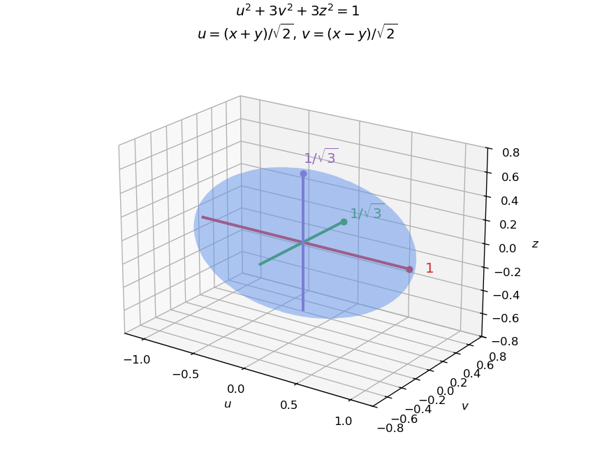
The diagonalized quadric is a prolate spheroid with semiaxes one and one over the square root of three
. Details. 
A diagonalizable matrix can certainly have exactly two distinct eigenvalues: is already diagonal and has an eigenbasis despite its repeated eigenvalue.
Past exam of the mathematics course of the year 2 of the natural sciences course of the University of Cambridge 2008 Paper 1 3 i Created 2026-10-18 Updated 2026-10-20
Past exam of the mathematics course of the year 2 of the natural sciences course of the University of Cambridge 2008 Paper 1 10 Solution Created 2026-10-18 Updated 2026-10-20
For nonzero with , the first variation of the Rayleigh quotient under isChoose fixed admissible homogeneous boundary conditions that make the variation boundary term vanish, such as zero endpoint values or zero endpoint derivatives. Compactly supported then show that a stationary function satisfies the Sturm-Liouville equation with . Conversely an eigenfunction satisfying those admissible conditions makes the variation zero. Multiplying its differential equation by and integrating by parts givesso the stipulated energy boundary term yields . The displayed energy condition alone is not a full specification of the admissible variations; it must be paired with boundary conditions for this variational equivalence.
For the final Dirichlet problem take the trial function , with . ThenThe Rayleigh-Ritz variational principle makes this an upper bound for the lowest eigenvalue. It is strictly above the true value: equality would require itself to be a lowest eigenfunction, but cannot vanish throughout for a constant . ThereforeAlthough the weight vanishes at the left endpoint, it is positive in the interior and its weighted quadratic norm is positive for every nonzero admissible continuous function; this does not obstruct the stated Dirichlet variational comparison.
There are unlisted articles, also show them or only show them.