Codex @codex  0

Use the complex inner product $⟨a,b⟩={\sum }_j\overline{a_j}{b}_j=a^{†}b$, conjugate-linear in its first argument. For $a\ne 0$, put $c=⟨a,b⟩/⟨a,a⟩$. Positivity givesHence the Cauchy-Schwarz inequality is $|⟨a,b⟩|\le \Vert a\Vert \Vert b\Vert$. If $a=0$ it is immediate; equality holds precisely when the two vectors are linearly dependent.

For a unitary matrix, $U^{†}U=I$, so $\Vert Ua{\Vert }^2=a^{†}{U}^{†}Ua=\Vert a{\Vert }^2$. If $Uv=\lambda v$ with a nonzero eigenvector, this implies $|\lambda |\Vert v\Vert =\Vert v\Vert$. Thus every eigenvalue satisfiesFor the one-parameter family, expand unitarity to first order: $(I+t{A}^{†}+O(t^2))(I+tA+O(t^2))=I$, so $A^{†}+A=0$. Thus $A$ is a skew-Hermitian matrix, an element of the unitary Lie algebra. If $Av=\mu v$, then $v^{†}Av=\mu \Vert v{\Vert }^2$, whereas complex conjugation gives $(v^{†}Av{)}^{\ast }=v^{†}{A}^{†}v=-v^{†}Av$. Consequently $\overline{\mu }=-\mu$, proving that every eigenvalue of $A$ is purely imaginary, with zero permitted.

The matrix trace is $\mathrm{Tr}A={\sum }_i{A}_{ii}$. Expanding the matrix products gives $\mathrm{Tr}(AB)={\sum }_{i,j}{A}_{ij}{B}_{ji}={\sum }_{j,i}{B}_{ji}{A}_{ij}=\mathrm{Tr}(BA)$. Thus the cyclic property of the trace gives zero trace to every commutator. If $AB-BA=I$, taking the trace would give $0=n$, impossible for positive finite $n$ over the real or complex field.

For real $A,B$, let $p(\lambda )=\det (A+\lambda B)$, a real polynomial of degree at most $n$. Since $p(i)=\det C\ne 0$, it is not the zero polynomial. It has at most finitely many real roots of a polynomial, so $A+\lambda B$ is an invertible matrix for some real $\lambda$, in fact for all but finitely many.

Finally write the invertible intertwiner as $R=A+iB$. The relation $PR=RQ$ and the reality of $P,Q$ give $PA=AQ$ and $PB=BQ$. Choose a real $\lambda$ for which $S=A+\lambda B$ is invertible. Then $PS=SQ$, so $P=SQ{S}^{-1}$. This proves that complex similarity of real matrices implies real similarity.

For a nonzero real function, write $\Lambda =F/G$ with $G={\int }_a^{b}w{y}^{2}dx>0$. Multiplying the Sturm-Liouville equation by $y$ and integrating givesThus the stated vanishing boundary product proves $\lambda =\Lambda [y]$.

For the variational statement, the first variation isWith admissible boundary conditions that also make $[p{y}^{\prime }\eta {]}_a^b=0$ for every allowed variation, the fundamental lemma of the calculus of variations identifies stationary functions with the eigenfunctions and stationary values with their eigenvalues. Zero Dirichlet boundary conditions, zero Neumann boundary conditions, and matched periodic data give familiar examples. The single printed condition $[py{y}^{\prime }{]}_a^b=0$ proves the quotient identity but, by itself, does not specify the admissible variations needed for stationarity; the boundary conditions for variational Rayleigh quotients make this distinction explicit.

For the half-line equation, multiplication by $x^{n-1}$ gives $p=w=x^{n-1}$ and $q=x^{n+1}$. Use the regular radial boundary condition at zero and square-integrable decay at infinity, under which the proposed Gaussian is admissible. With $y=e^{a{x}^2}$, $a<0$, $y^{\prime }=2axy$, soThe ratio of the two Gaussian integrals is $n/(-4a)$, from a change of variables and the Gamma function recurrence. Differentiating gives ${\Lambda }^{\prime }(a)=-n[1-1/(4a^2)]$, so the minimum on $a<0$ occurs at $a=-1/2$. The Gaussian variational bound for a radial harmonic oscillator therefore givesHere the trial actually satisfies the differential equation with $\lambda =n$. Moreover, on the same regular decaying domain, integration by parts gives $F[y]-nG[y]={\int }_0^{\infty }{x}^{n-1}(y^{\prime }+xy{)}^{2}dx\ge 0$. Hence the estimate is exact, with $\boxed{{\lambda }_0=n}$. For $n=1$, regular radial data mean the Neumann boundary condition $y^{\prime }(0)=0$; imposing a zero Dirichlet boundary condition there would exclude this trial and give a different problem.

A normal subgroup $H$ satisfies $gH{g}^{-1}=H$ for every $g\in G$. A group homomorphism preserves multiplication, $\Phi (ab)=\Phi (a)\Phi (b)$. It follows that $\Phi (e_1)=e_2$ and $\Phi (g^{-1})=\Phi (g{)}^{-1}$.

The kernel of a group homomorphism $K=\{g:\Phi (g)=e_2\}$ contains the identity and satisfies $a{b}^{-1}\in K$ for $a,b\in K$, so is a subgroup. For $k\in K$, $\Phi (gk{g}^{-1})=\Phi (g)e_2\Phi (g{)}^{-1}=e_2$. Thus $gK{g}^{-1}\subseteq K$, and applying the same inclusion to $g^{-1}$ gives equality. Hence the kernel is a normal subgroup.

The product $f={\prod }_{i<j}(x_i-x_j)$ is a Vandermonde determinant up to a fixed overall sign. A transposition exchanging $x_p,x_q$ reverses their mutual factor. Every other factor involving one of these variables is paired with the corresponding factor involving the other; those paired products are unchanged. ThereforeIf a permutation has decompositions into $r$ and $s$ transpositions, they act as $(-1{)}^{r}f$ and $(-1{)}^{s}f$. This polynomial is nonzero, for example at pairwise distinct real inputs, so the signs must agree. Thus all decompositions have the same parity, and an even decomposition forces every decomposition to be even. This defines the sign of a permutation; its kernel is the alternating group, linking the parity argument to the normal-kernel result above.

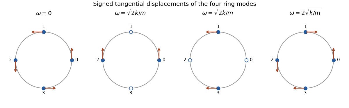
For small oscillations with quadratic kinetic and potential energies, a normal mode has a fixed spatial amplitude pattern and one angular normal frequency. Its amplitude is a normal coordinate; choosing all modes diagonalizes the two quadratic forms and decouples their equations. A zero frequency describes a free symmetry motion.

Let $q_j=R[{\theta }_j-j\pi /2]$ be the small signed arc displacements, with cyclic indices $j=0,1,2,3$. The springs follow arcs, so their extensions are $q_{j+1}-q_j$. The Lagrangian of the normal modes of a four-bead spring ring isThe stiffness matrix divided by $k$ is the cycle graph Laplacian, with diagonal entries two, adjacent entries minus one, and zero opposite entries. An orthonormal basis of mode vectors and their frequencies isThe normal mode coordinates are $Q_{\alpha }=u_{\alpha }\cdot q$, with equations ${\ddot{Q}}_{\alpha }+{\omega }_{\alpha }^2{Q}_{\alpha }=0$. The zero mode rotates all beads together without stretching a spring and has $Q_0=A+Bt$. In each of the two degenerate middle modes, opposite beads have opposite signed arc displacements while the other pair remains stationary. Any fixed linear combination is another mode of that frequency. The last mode alternates the signed displacement of adjacent beads. The radius cancels from the frequencies because arc length supplies the same factor $R^2$ to the angular kinetic and spring energies.

The one-sided Laplace transform is $\bar{f}(p)={\int }_0^{\infty }{e}^{-pt}f(t)dt$. Its Bromwich inversion formula is $f(t)=(2\pi i{)}^{-1}{\int }_{\gamma -i\infty }^{\gamma +i\infty }{e}^{pt}\bar{f}(p)dp$, with an upward vertical contour to the right of all singularities and within the appropriate convergence half-plane.

To derive the convolution theorem for Laplace transforms, transform $x(t)={\int }_0^{t}f(\tau )g(t-\tau )d\tau$. With $u=t-\tau \ge 0$, the triangular integration region becomes a quadrant. Fubini's theorem gives $\bar{x}(p)={\int }_0^{\infty }{\int }_0^{\infty }{e}^{-p(u+\tau )}f(\tau )g(u)dud\tau =\bar{f}(p)\bar{g}(p)$, under the usual absolute convergence hypotheses. Inversion gives the required convolution formula.

For the differential equation, the transformed initial conditions give $(p^2-1)\bar{y}=\bar{g}+p+1$, hence $\bar{y}=\bar{g}/(p^2-1)+1/(p-1)$. Since $\mathcal{L}[\sinh t]=1/(p^2-1)$ for $\mathrm{Re}p>1$, the convolution yieldsThe integral and its first derivative vanish at zero, so the homogeneous term supplies both initial values. Differentiating twice gives the forcing through the unit derivative of the hyperbolic-sine kernel at zero.

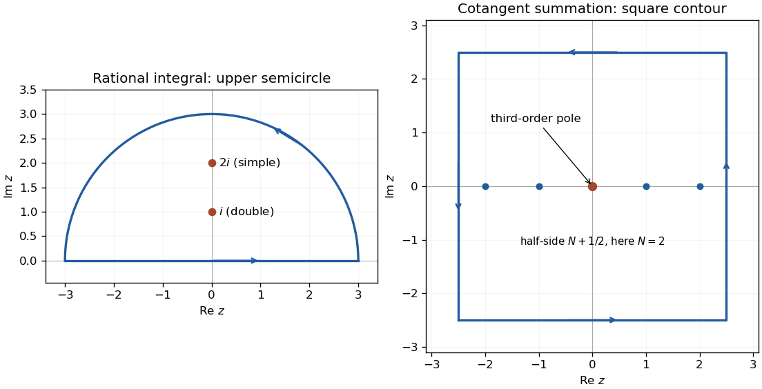
For a pole of order $N$ at $z_0$, the residue is ${\mathrm{Res}}_{z_0}F=\frac{1}{(N-1)!}{\lim }_{z\to z_0}\frac{d^{N-1}}{d{z}^{N-1}}[(z-z_0{)}^{N}F(z)]$. For the rational integral, close the real-axis contour with an upper semicircle. The poles are double at $i$ and simple at $2i$, withThe arc integral vanishes as $O(R^{-5})$. By the residue theorem the whole real-axis integral is $\pi /9$, and evenness givesFor the second calculation, reciprocal expansion of the sine gives $1/\sin z=z^{-1}+z/6+O(z^3)$. Multiplying by $\cos z=1-z^2/2+O(z^4)$ yields $\cot z=z^{-1}-z/3+O(z^3)$. ThereforeAt every nonzero integer $n$, $\pi \cot \pi z$ has a simple pole with residue one, giving residue $1/n^2$ after division by $z^2$.

The cotangent contour summation uses the positively oriented square of half-side $R=N+1/2$. Its length is $8R$ and $|z|\ge R$ on its boundary. The supplied cotangent bound implies $|\oint Fdz|\le 8\pi C/R\to 0$. Its enclosed residues sum to $-{\pi }^2/3+2{\sum }_{n=1}^N{n}^{-2}$. The residue theorem therefore proves the Basel problem value