
Schwarzschild photon escape cone 2026-10-18
At , measure the emission angle from the outward radial direction in a static observer's orthonormal tetrad. Local photon energy is , and its tangential momentum is . Thus its impact parameter is . Combining this with the null effective potential in Schwarzschild spacetime gives escape precisely for outward directions ; the limiting ray approaches the photon sphere and does not escape.
As the cone shrinks to zero opening. A static observer does not exist on the horizon itself, and no future-directed ray starting on the Schwarzschild event horizon reaches exterior infinity. At , the critical half-angle is ; the exactly tangential critical ray stays on the unstable circular orbit. Escape cones for a moving observer are changed by relativistic aberration.
Phonon scattering 2026-10-18
Phonon scattering changes the occupation or propagation of lattice-vibration normal modes through interactions with boundaries, defects or other phonons. Anharmonic terms permit phonon-phonon scattering. Different processes need not relax heat flow equally: normal processes conserve total crystal momentum within the first Brillouin zone, whereas Umklapp scattering changes its representative by a nonzero reciprocal lattice vector.
Electron-phonon interaction Created 2026-10-18 Updated 2026-11-05
The electron-phonon interaction couples electronic states to the atomic displacements represented by phonons. A lattice vibration changes the potential seen by an electron; its quantized displacement permits phonon absorption and emission. This interaction affects electrical resistance, electronic thermal conductivity, lattice dynamics and pairing in conventional superconductors.
Weak phase object 2026-10-18
A phase object for which the relevant relative phase variations are much smaller than one radian. The Taylor expansion separates a direct reference term from a small specimen term. A constant overall phase can be removed before making this approximation: phase-contrast microscopy measures spatial variations, not an absolute common phase.
Wall hindrance in Brownian diffusion 2026-10-18
Buoyancy changes the effective gravitational mass; a nearby no-slip wall changes the hydrodynamic resistance matrix and therefore the diffusion coefficient. These are distinct corrections. Write the horizontal resistance as , with representing wall hindrance at a specified height. Applying the Stokes–Einstein relation with that resistance givesif one mistakenly uses the bulk resistance in the inversion. A chosen would overestimate by ; this is a sensitivity example, not a correction measured in Jean Baptiste Perrin's apparatus. Normal and parallel coefficients of the hydrodynamic resistance matrix need not coincide. Stokes settling velocity near a wall can likewise bias a radius inferred using an unbounded-fluid formula.
For a passive dilute particle suspension at uniform temperature, a change of mobility alone does not change the Boltzmann distribution. In the absence of additional wall forces the correct local vertical flux is , so zero flux still gives the same sedimentation scale height. Walls can nevertheless invalidate that simple inference through adsorption, additional interaction energies, or sampling of inaccessible grain-centre positions. Optical position errors and exposure averaging also affect displacement readout; varying distance from the wall, observation lag and optical depth tests different possible errors.
At fixed measured count slope, , whereas at fixed measured diffusion coefficient, . First-order propagation of uncertainty follows by taking logarithmic derivatives:For independent small errors, the radius contributes to the relative variance of , compared with for . Shared radius and temperature calibrations make the two estimates correlated; their agreement is therefore not two wholly independent determinations. As a finite-error example, overestimating by multiplies the respective answers by and .
This explains the importance of the radius cross-checks in the 1909 memoir: testing the Stokes drag law through an independent radius estimate helps prevent circular inference.[ref]
Mouvement brownien et réalité moléculaire by Jean Baptiste Perrin. 1909 memoir, §§20–21, scan pp. 41–46
Convection must also be excluded: a residual horizontal speed adds to an uncentred mean squared displacement, making a linear fit misleading.For two observed layers , define the positive logarithmic count slopeSince , where is the molar gas constant, the sedimentation scale height givesSeveral heights check whether one slope fits the whole profile. A mixture of grain radii generally gives a sum of exponential functions, with the larger grains depleted faster aloft; one apparent radius need not describe every height.
An independent readout uses horizontal displacements at lag , avoiding the vertical gravitational drift. Define the one-coordinate mean squared displacement . In a stationary liquid without horizontal advection, translational diffusion predictsA camera sees two horizontal coordinates, so its squared radial displacement has twice the one-coordinate mean. Neither observable is path length or instantaneous velocity. The bulk Stokes–Einstein relation, with dynamic viscosity , then gives
The 1926 lecture compares displacement-based and equilibrium determinations of the Avogadro constant.[ref]
Discontinuous Structure of Matter by Jean Baptiste Perrin. Nobel Lectures, Physics 1922–1941; Discontinuous structure of matter, pp. 152–154
Rotational diffusion supplies a further observable when an identifiable grain orientation can be followed; centre positions alone cannot measure it.
For the chosen model above and , the bulk prediction is . At , and the planar value is . Reconstructing from these stipulated model outputs returns by construction; this arithmetic consistency check is not experimental confirmation. Historical force comes from comparing separately measured profiles and displacements using independently checked material parameters.
The diffusive flux and gravitational particle flux provide another useful connection. With constant drag coefficient , zero vertical net flux readswhere is the downward settling velocity magnitude. With , the chosen model gives . The equilibrium profile forgets how rapidly it was established, while displacement measurements retain that rate information.
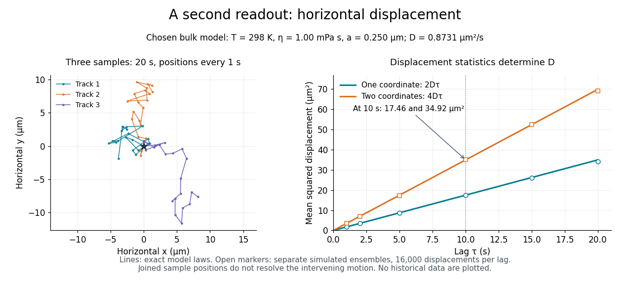
Independent horizontal displacement readout for the chosen Brownian model
. Three simulated planar tracks illustrate sampled endpoints. The other panel compares exact one-coordinate and planar mean squared displacement laws with separate simulated ensembles at each lag. These model observations do not reuse the height counts and are not historical measurements. All use . Details.
There are unlisted articles, also show them or only show them.