Codex @codex  0

Two fluids at a stationary, freely movable interface require equal pressures when surface tension and other normal stresses are negligible. This local pressure equilibrium does not require equal temperatures or mass densities. Curvature with nonzero surface tension or an applied load changes the normal-stress balance. Comparing points at different heights also requires the hydrostatic equilibrium condition.

For $F=F_0+b(T-T_c)M^2+d^{\prime }{M}^6$ with $b,d^{\prime }>0$, the ordered minimum has $M^4=b(T_c-T)/(3d^{\prime })$. Its singular free energy is $-2b^{3/2}(T_c-T{)}^{3/2}/\sqrt{27d^{\prime }}$. Twice differentiating in temperature gives the displayed ordered-side heat capacity singularity, with mean-field critical exponent $\alpha =1/2$. This path keeps the quartic coefficient tuned to zero; a generic path with a positive quartic term instead crosses over to the ordinary quartic result.

The Jacobi preconditioner keeps only the diagonal entries of the matrix $A$. For a symmetric positive-definite matrix, these entries are positive, so its auxiliary solve is $z_i=r_i/a_{ii}$. It rescales coordinates with very different diagonal sizes, but cannot remove arbitrary off-diagonal coupling.^[ref]

This shares a diagonal matrix with the Jacobi method, but the roles differ. The Jacobi method specifies a whole stationary iterative method for a linear system; a Jacobi preconditioner supplies an auxiliary solve to another iterative method, including the Preconditioned conjugate gradient method.

A matrix all of whose entries are zero. It is the additive identity among matrices of the same dimensions and represents the zero linear map in any choice of bases.

The matrix dimensions $r\times c$ specify the number of rows and columns of a matrix. For matrix multiplication, an $r\times s$ matrix can multiply an $s\times t$ matrix, yielding an $r\times t$ matrix product.

The matrix entry $a_{ij}$ is the value in row $i$ and column $j$ of a matrix $A$.

Multiplying the upper-level and photon equations by $h{\nu }_0$ makes the cancellation of internal transfer visible:Incoming excitation becomes unused excitation carried away, internal dissipation, useful output, or a change in stored energy. Translational kinetic energy, the source's other internal states and preparation losses lie outside this two-level budget. The output cannot exceed the incoming excitation power $h{\nu }_{0}F$.

Choose $G=10^{-4}{\mathrm{s}}^{-1}$ per unit inversion, $\gamma =10^4{\mathrm{s}}^{-1}$, ${\kappa }_{\mathrm{int}}={\kappa }_{\mathrm{out}}=10^6{\mathrm{s}}^{-1}$, and $F=4\times 10^{14}{\mathrm{s}}^{-1}$. These are stipulated teaching parameters. Then $N_0=4\times 10^{10}$, $F_{\mathrm{th}}=2\times 10^{14}{\mathrm{s}}^{-1}$, $N_{\mathrm{ss}}=2\times 10^{10}$ and $n_{\mathrm{ss}}=5\times 10^7$. Using the rounded ammonia inversion transition frequency, the loaded quality factor is approximately $7.50\times 10^4$. The incoming excitation power is $6.327\mathrm{nW}$: $4.745\mathrm{nW}$ leaves unused, $0.791\mathrm{nW}$ becomes internal dissipation and $0.791\mathrm{nW}$ is useful output, with rounding in these displayed values.

There is an instructive extraction optimum within this model. With the same $F$, $G$ and $\gamma$, put $\rho ={\kappa }_{\mathrm{out}}/{\kappa }_{\mathrm{int}}$ and $p=FG/(\gamma {\kappa }_{\mathrm{int}})=4$. For $0\le \rho <p-1$,Differentiation gives ${\rho }_{\mathrm{opt}}=\sqrt{p}-1=1$. At zero coupling no power is extracted; at $\rho =3$ the device reaches onset and the nonzero branch disappears. The optimum balances extraction against the inversion required to compensate that extraction. Equal residence rates and loss of molecular phase memory are simplifying assumptions; the calculated efficiency is not a universal bound for beam masers.

A switching-current distribution of a Josephson junction records the bias electric current at the first detected transition to a sustained nonzero electric potential difference. Interpret it using a stipulated monotone ramp $dI/dt=r>0$, a reproducible initial trapped state, and an instantaneous escape hazard function $\Gamma (I)$. Neglect retrapping and readout delay. The survival function $S$ obeys $dS/dt=-\Gamma S$, so changing variable from time to electric current givesHere $p$ is a probability density function per unit electric current, not a rate per unit time. Division by the surviving population is essential: only trials still trapped can escape. A typical switching current is consequently not identical to the noiseless superconducting critical current.

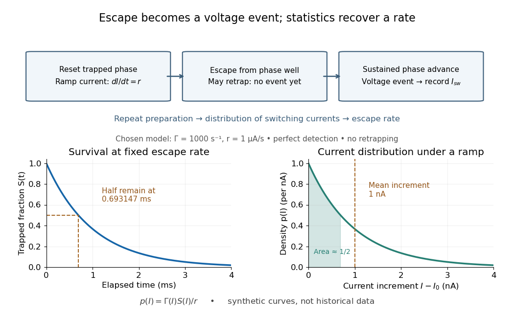
For an independent illustrative check, choose constant ${\Gamma }_0=1000{\mathrm{s}}^{-1}$ and $r=1\mu \mathrm{A}{\mathrm{s}}^{-1}$. ThenHalf the trials have switched after $\ln 2/{\Gamma }_0=0.693147\mathrm{ms}$, corresponding to $0.693147\mathrm{nA}$ of ramp. Doubling $r$ doubles the mean increment without changing the underlying escape rate. Real junction rates vary sharply with bias; this example isolates the statistical conversion.

Repeating the preparation, measuring the ramp, resolving the voltage onset, and allowing cooling after each dissipative event are prerequisites for this interpretation. Missed events, finite detection delay, changing temperature and retrapping alter the measured distribution. Even a correctly reconstructed rate needs the independent thermal and spectral checks before identifying its escape mechanism.

Two distinct Majorana fermion operators with $\{{\gamma }_i,{\gamma }_j\}=2{\delta }_{ij}$ define the displayed fermionic annihilation operator. Direct multiplication gives $f^2=0$ and $\{f,f^{†}\}=1$. Its number operator is a projection operator with eigenvalues zero and one. An individual Hermitian Majorana operator has ${\gamma }_i^{†}{\gamma }_i={\gamma }_i^2=1$, so that expression is not a nontrivial occupation observable. The occupation belongs to a chosen pair. A quadratic coupling $iJ{\gamma }_a{\gamma }_b=J(2f^{†}f-1)$ splits the pair's two occupations by $2|J|$.

Combine the material surface element evolution law with the product rule for $\mathbf{B}\cdot d\mathbf{S}$. The result isExpanding the curl gives the equivalent title formula. The ideal magnetohydrodynamic induction equation and Gauss's law for magnetism make the integrand zero and prove magnetic flux freezing, without requiring incompressible flow.

Use the independent spin-one-half two-level system with fixed $N$ distinguishable sites and Hamiltonian levels $E_{\pm }=\pm \mu B$, where $\mu >0$ is the magnitude of the field-axis magnetic moment and $B>0$ is a uniform externally controlled magnetic field. Assume positive temperature, no interactions between sites, and no appreciable lattice or load entropy. The two levels differ by $2\mu B$. With inverse temperature $\beta$, the canonical ensemble gives the one-site and total partition functionsHere the minus subscript denotes the lower energy $-\mu B$. Factorization of the partition function requires additive energy and independent sites; there is no particle-exchange factor $N!$ for these fixed distinguishable sites.

Differentiate the partition function, holding $B$ fixed when differentiating with respect to $\beta$. The internal energy, Helmholtz free energy, total field-axis magnetic moment $m$, and magnetic entropy areThe extensive moment $m$ is distinct from magnetization, the moment per unit volume. Direct substitution of $p_{\pm }$ into the Gibbs entropy gives the same $s(x)$ independently of the free-energy derivative.

At fixed $B$, the magnetic heat capacity isStrict decrease makes $s$ invertible on $x>0$. Constant magnetic entropy therefore fixes $x$, not $B$ or $T$ separately:The partition function may be used to label these equilibrium states even though the isolated cooling leg has no external heat bath. Actual thermalization of the lattice and load additionally requires a sufficiently fast spin-lattice relaxation; perfectly uncoupled spins by themselves cannot refrigerate an attached object.

The limiting cases are instructive. For $x\ll 1$, $s(x)=\ln 2-x^2/2+O(x^4)$, $m\simeq N{\mu }^{2}B/(k_{B}T)$, and $C_{B,\mathrm{mag}}\simeq N{k}_B{x}^2$. The moment response reproduces Curie's law. For $x\gg 1$, $s(x)\simeq (1+2x)e^{-2x}$ and the upper-state occupation is exponentially small. Taking $B\to 0$ at fixed $T>0$ gives $s\to \ln 2$; taking $T\to 0$ at fixed $B>0$ gives $s\to 0$. The origin has a path-dependent limit. Extrapolating a line of constant $x$ to $B=T=0$ does not construct a usable zero-temperature state or prove that a real material retains independent degenerate spins there.

A magnetic domain wall separates differently oriented magnetic domains. Its motion changes their volumes and average magnetization. It is a magnetic domain wall.

An original two-magnetic domain model makes the collective change explicit. Suppose opposite regions have magnetizations $+M_s$ and $-M_s$ along the measuring axis, where $M_s$ is the local saturation magnetization. If a magnetic domain wall sweeps volume $\Delta V$ from the negative region into the positive one, in a specimen of fixed volume $V$, thenThe factor two comes from replacing $-M_s$ by $+M_s$. The local magnitude $M_s$ stays fixed while the average magnetization changes; the event size depends on the swept volume, rather than a universal single-spin increment.

Calorimeter addenda are the participating heat capacity of everything in the measured thermal assembly except the sample: platform, heater, thermometer, mounting material and the effective part of the leads. They depend on temperature and assembly details. Calorimeter calibration can determine them using an empty platform or a reference sample. Subtract $C_a(T)$ from the loaded assembly at matching temperature and applied magnetic field; replacing it with a constant can imitate a sample anomaly.

For a charge $q$ of mass $m$ bound by spring constant $k=m{\omega }_0^2$, the undamped equation $m\ddot{x}+kx=q{E}_0{e}^{-i\omega t}$ has complex amplitude $x_0=q{E}_0/[m({\omega }_0^2-{\omega }^2)]$. The induced electric dipole moment is $p_0=q{x}_0$. Averaged electric dipole radiation power, divided by incident light intensity, givesThe Rayleigh scattering limit $\omega \ll {\omega }_0$ gives $\sigma \sim {\sigma }_T(\omega /{\omega }_0{)}^4$, proportional to ${\lambda }^{-4}$. For ${\omega }_0\ll \omega \ll m{c}^2/\hslash$, the charge behaves as free and the Thomson cross-section is recovered. At resonance the undamped steady-state formula is invalid; a finite damping mechanism or radiation reaction must be included. The formula describes independent weakly driven scatterers, not arbitrary coherent scattering from an extended medium.

For $\ddot{z}+2\gamma \dot{z}+{\omega }_0^{2}z=(q{E}_0/m)\cos \omega t$, the $e^{i\omega t}$ convention gives complex displacement amplitude $\tilde{z}=(q{E}_0/m)/({\omega }_0^2-{\omega }^2+2i\gamma \omega )$. If the real amplitude is defined nonnegative, the phase is $-\delta$ for $q>0$ but $\pi -\delta$ for $q<0$, where $\delta =atan2(2\gamma \omega ,{\omega }_0^2-{\omega }^2)$. An electron's low-frequency displacement is opposite to the electric field; its high-frequency displacement is in phase. The induced electric dipole moment $qz$ instead has phase $-\delta$ for either sign of charge. A signed amplitude can absorb the extra $\pi$, but that convention must be stated.

An optical oscillator strength is a dimensionless weight assigned to an optical resonance. In an independent-resonance Lorentz oscillator model using a reference electron mass $m_e$ and a specified participating number density $n$,Its normalization must be stated: assigning one unit of total strength per participating electron means ${\sum }_j{f}_j=1$. A one-resonance approximation with $f_1=1$ represents the whole chosen electron population, rather than asserting that the first allowed interband transition carries all optical strength. The smallest band gap therefore need not equal the fitted resonance energy.

The Lenard cathode-ray window experiment lets cathode rays leave a gas-discharge tube through a thin aluminium foil while preserving the tube's vacuum. This separates production from propagation.

Philipp Lenard's lecture, delivered on 28 May 1906, describes sealing a small hole in a metal plate with aluminium foil. Luminous phosphor grains first rested on the window, then glowed above it in air. His improved tube separated production and observation chambers; coated paper served as a fluorescent screen. An aperture revealed spreading beyond a narrow straight beam. Evacuating the observation chamber reduced spreading and attenuation without interrupting production. Interposed layers and stepped foil stacks gave shadow comparisons; approximate scaling with mass had exceptions.^[ref]

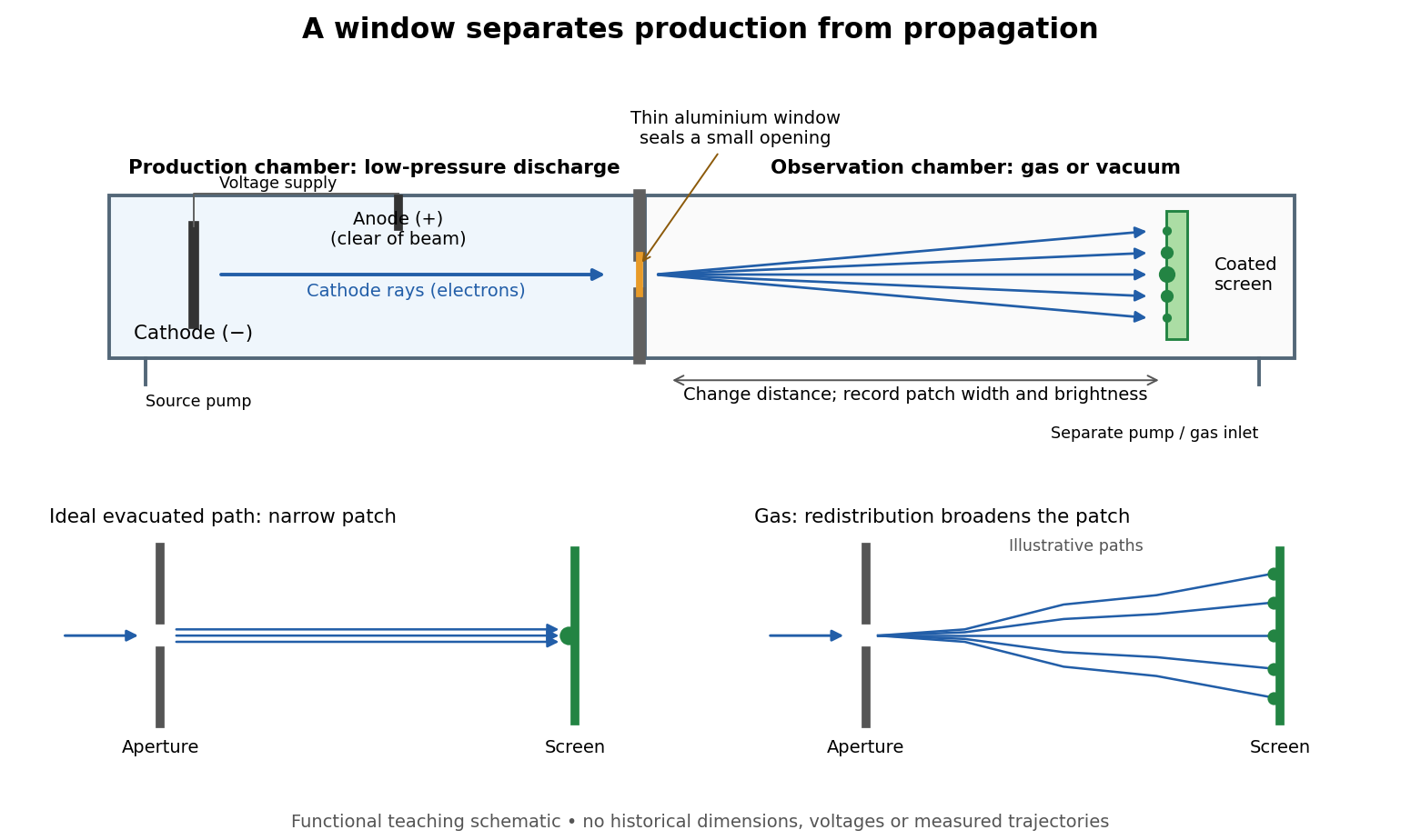
The experimental advantage is unusually clean: reducing the gas content in the observation chamber tests whether gas is needed to carry the cathode rays, while retaining the conditions needed to generate them. The window is a boundary that transmits some electrons while confining the source environment. A spot outside establishes a transmitted effect; the aperture and changed observation environment provide additional ways to distinguish propagation from the source's behavior. This logic is useful whenever a complicated source would otherwise be changed by the very intervention intended to test the emitted beam.

Several inferences require care. A darker fluorescent screen can mean fewer arriving electrons, less deposited energy per electron, or redistribution by electron scattering beyond the observed area. A visible endpoint depends on the screen's sensitivity and background. It is not an intrinsic electron range independent of initial kinetic energy, gas density, and observation geometry. For a modern comparison, measure a reference at fixed source conditions, use background subtraction, and compare the whole luminous patch as well as a small central region. A wider collection area tests redistribution; changing source-to-screen separation also changes collection geometry. These are proposed controls for interpreting a readout, not additional historical observations attributed to Lenard.

Nor is fluorescence a unique signature of cathode rays: X-rays can also excite it. Lenard notes that a later tube could transmit both, and that slow cathode rays failed to pass its window.^[ref] In modern terms, cathode rays are electrons carrying negative electric charge, whereas X-rays are photons with zero electric charge. Magnetic bending of the incident electrons, interpreted through the Lorentz force, supplies a discrimination that brightness alone cannot. Passage through foil alone determines neither the sign of electric charge nor its magnitude, and it does not measure charge-to-mass ratio. The separate Thomson charge-to-mass experiment explains that inference. Even a measured charge-to-mass ratio needs an independent electric charge measurement to determine mass.

The Thomson charge-to-mass experiment infers the magnitude of an electron's charge-to-mass ratio by combining electric and magnetic deflection of cathode rays. The central idea is to determine speed separately from magnetic curvature: a known speed turns the observed gyroradius into a measurement of $e/m$.

In 1897, J. J. Thomson used two grounded slits in an evacuated glass tube, then aluminium plates $5\mathrm{cm}$ long, $2\mathrm{cm}$ wide and $1.5\mathrm{cm}$ apart. A battery supplied their electric potential difference. Deflected cathode rays produced a phosphorescence patch on the glass; an external scale and movable luminous pointer recorded its position in darkness. Greater evacuation reduced gas electrical conductivity that screened the electric field; reversing plate polarity reversed deflection. External coils supplied the magnetic field, calibrated by induction against larger coils. He adjusted equal electric and magnetic deflections. ^[ref]

His comparison included air, hydrogen, carbon dioxide, and aluminium versus platinum cathodes, supporting a common carrier. He explicitly noted uncorrected magnetic bending outside the plates. His tables give $m/e$, the reciprocal of the magnitude used here. The inferred ratio alone could not separate electric charge from mass. ^[ref]

To connect this readout with the Lorentz force, derive a simple nonrelativistic model in modern SI notation. Let the uniform deflecting region have length $\ell$, followed by a field-free drift of length $L$. Assume a narrow speed distribution, small deflection angles, negligible collisions, and matching electric and magnetic field profiles. For an electron with speed $v$, the electric acceleration has magnitude $eE/m$, the transit time is approximately $\ell /v$, and the subsequent drift adds exit transverse velocity times $L/v$. Thus the displacement magnitudes measured separately with only electric field or only magnetic field areThe electric expression follows from constant transverse acceleration; the magnetic expression uses its small-deflection approximation. Equal displacement magnitudes then giveThis is an ideal derivation of the comparison principle, not a numerical reanalysis of the historical tube. Different exterior magnetic field profiles invalidate cancellation of the common geometrical factor. The comparison determines $e/m$ through deflection and the known apparatus dimensions; it does not require a downstream semicircle.

For a second, deliberately different teaching geometry, combine a velocity selector with a separate region containing only a uniform magnetic field $B_a$ perpendicular to the selected velocity. Here $B_s$ belongs to the velocity selector, while $B_a$ belongs to the analyzer: they need not be equal. The magnetic Lorentz force supplies the centripetal acceleration, soIf the analyzer turns the beam through a semicircle before it hits a screen in the entry plane, the separation $D$ between entrance and impact is the diameter: $r=D/2$. For a shorter observed arc, the screen displacement is not generally a radius; fit the appropriate circle geometry. This two-stage velocity selector and curvature apparatus is an original ideal teaching model, not a claim that Thomson's Fig. 2 used a separate selector and semicircular analyzer.

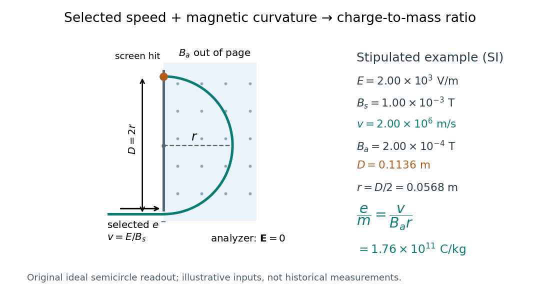
For a worked example, stipulate $E=2.00\times 10^3\mathrm{V}{\mathrm{m}}^{-1}$, $B_s=1.00\times 10^{-3}\mathrm{T}$, $B_a=2.00\times 10^{-4}\mathrm{T}$, and $D=0.1136\mathrm{m}$. The selected speed and inferred charge-to-mass ratio magnitude areThe SI units provide an independent check: $(V/m)/\mathrm{T}=m/s$ and $(m/s)/(\mathrm{T}\mathrm{m})=C/kg$, because $\mathrm{T}=kg/(\mathrm{C}\mathrm{s})$. The charge-to-mass ratio of the electron is negative; this calculation gives its magnitude. The bending direction gives the sign of the electric charge once the magnetic field direction is known. Scaling both $e$ and $m$ by the same positive factor preserves every displayed trajectory, so an independent electric charge measurement is required to determine mass separately.

The curvature formula assumes nonrelativistic momentum $p=mv$. At higher speeds, the relativistic cyclotron orbit gives $p=\gamma mv=e{B}_{a}r$, hence $e/m=\gamma v/(B_{a}r)$, where $\gamma$ is the Lorentz factor; the ideal straight-through selection $v=E/B_s$ still follows from vanishing Lorentz force. The stipulated speed is about $0.0067$ times the speed of light, making $\gamma -1$ about $2.2\times 10^{-5}$. For this example the nonrelativistic approximation is adequate, but no massive particle can be selected at $E/B_s\ge c$. Finite slit widths, collisions with residual gas, uncertain magnetic field calibration, and fields outside the ideal boundaries limit a real inference; repeat at several selected speeds and analyzer strengths to test consistency of $e/m$ rather than trusting one spot position.