
Velocity selector Created 2026-10-18 Updated 2026-10-20
A velocity selector uses perpendicular electric field and magnetic field to transmit a narrow range of speeds along a chosen beam direction. Assume uniform static electric field and magnetic field , with , and an incident velocity . The cross product gives , so the transverse Lorentz force isFor an electron, the electric force points downward and the magnetic force upward. A faster electron initially bends upward; a slower one initially bends downward. At the selected speed, both forces cancel along the whole straight trajectory. The cancellation is independent of mass and nonzero electric charge; it selects velocity, not a particular charge-to-mass ratio. A component of velocity parallel to the magnetic field is not constrained by the cancellation, so the incident beam must also have its direction restricted.
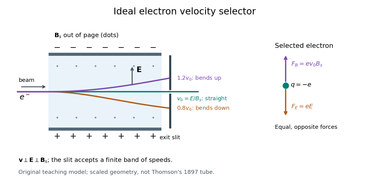

A real exit slit accepts a finite range of speeds and incident directions. A zero displacement at one screen alone does not establish zero force throughout the path: a curved trajectory could return to that screen position. The ideal velocity selector interpretation requires a straight aligned beam, known overlapping electric field and magnetic field, and sufficiently narrow entrance and exit slits. Its useful role in the Thomson charge-to-mass experiment teaching model is to supply speed independently of the subsequent magnetic bending.
Charge-to-mass ratio Created 2026-10-18 Updated 2026-10-20
The charge-to-mass ratio is a body's electric charge divided by its mass . Its SI unit is the coulomb per kilogram, . In a prescribed electric field and magnetic field, nonrelativistic acceleration depends on through the Lorentz force. Two bodies with the same initial position, velocity, and charge-to-mass ratio therefore have the same trajectory in this ideal model. For an electron, write with the elementary charge: , whereas the positive number is the magnitude of the charge-to-mass ratio.
Magnetic rigidity Created 2026-10-18 Updated 2026-10-20
Magnetic rigidity measures the resistance of a charged particle's momentum to bending by a magnetic field. The relativistic cyclotron orbit gives , where is the transverse gyroradius. For motion perpendicular to a uniform magnetic field, is the whole momentum. A measured magnetic rigidity fixes momentum per magnitude of electric charge; it does not by itself fix mass, kinetic energy, or the sign of the electric charge. This distinction makes the Anderson positron track experiment an especially revealing application of the Lorentz force.
For a free massless real scalar field with wave speed set to one and metric , define and . Its symmetric stress-energy tensor is . The Lorentz current has density and flux . Its conserved charge is the displayed expression when boundary flux vanishes. In one spatial dimension it generates boosts, not spatial rotations; there is no independent purely spatial angular-momentum component. Its conservation says that the center of energy moves uniformly. This is a symmetry of the wave-field model and need not survive boundaries or additional material effects.
Participation ratio 2026-10-18
For an eigenvector normalized by , the participation ratio in its site basis isIt estimates how many sites carry appreciable probability. Equal weight on sites and zero elsewhere gives , irrespective of their wave phases. A single occupied site gives ; uniform probability on all sites gives . These are exact constructed examples, not claims about particular Hamiltonian operators.
To prove the bounds, write . Since , , giving . The Cauchy-Schwarz inequality gives , giving . Thus the measure has useful limits without assuming an exponential shape. Comparing as increases helps distinguish a state filling the sample from one occupying a fixed region, provided energy selection and disorder statistics are controlled.
Localization length 2026-10-18
The localization length measures the decay scale of a localized eigenstate's wave amplitude envelope. Here is the site spacing and its centre. With this amplitude convention, probability decays on half that scale:Individual random tails fluctuate; this notation describes their typical envelope, not exact equality at every site. A localization length much greater than a finite sample's length makes a state look extended inside that sample. The participation ratio below is an effective site count, not an independent fitted value of .
Log-linear exponential-decay fit Created 2026-10-18 Updated 2026-10-25
An exponential decay rate becomes a straight line in and , where is a fixed reference rate. Constant small fractional rate errors become approximately constant vertical errors by propagation of uncertainty. With independent Gaussian log-rate errors, linear least squares gives and .
The covariance matrix is obtained by applying the variance rules to these linear estimators:Transforming back gives , , and . If a candidate lifetime fixes the slope , the intercept must be refitted as . The profiled objective obeysThis follows by separating the centred slope residual from the unrestricted regression residual, whose inner product with the design columns is zero by the normal equations for linear least squares. Known supplied measurement errors are not rescaled by the observed reduced chi-squared. This log-error model is an approximation for proportional errors, not an exact replacement for every raw-count likelihood.
Mass attenuation coefficient Created 2026-10-18 Updated 2026-10-20
The linear attenuation coefficient divided by the material mass density.
Wall-plug efficiency 2026-10-18
The emitted optical power divided by electrical input power. For the bare-device calculation in light-emitting diode efficiency, ; a complete lamp also consumes power in its driver. Luminous efficacy, measured in lumens per watt, additionally weights the spectrum by human visual sensitivity and is a different quantity.
Light extraction efficiency 2026-10-18
External quantum efficiency 2026-10-18
Internal quantum efficiency Created 2026-10-18 Updated 2026-10-20
For the convention used in light-emitting diode efficiency, the internally generated photon rate divided by the rate of electron and electron hole pairs reaching the emitting layer. Its denominator must be stated when comparing measurements.
Liénard-Wiechert field Created 2026-10-18 Updated 2026-11-05
The Liénard-Wiechert field is the electric field and magnetic field obtained from the retarded potentials of a moving point charge. In the nonrelativistic radiation zone, the electric radiation field is at retarded time. Its outgoing Poynting vector integrates to the Larmor formula. Coulomb and induction fields must also be retained when a near-field calculation is required.
State-counting and helicity factors in pion decay Created 2026-10-18 Updated 2026-11-05
In a box-normalized treatment of negative-pion two-body decay with a massless antineutrino, . The simple density of states is therefore proportional to . The spin-zero two-body helicity selection requires positive charged-lepton helicity, whose left-chiral weight is . Since , the energy factors cancel in the product and give the standard relative rate proportional to . A Lorentz-invariant phase-space measure distributes normalization factors differently but gives the same observable ratio when the amplitude is normalized consistently.
Sharp bounds from binary conditional probabilities Created 2026-10-18 Updated 2026-10-25
Write , and . The law of total probability gives the displayed convex combination. With fixed and free in ,With fixed and free in ,The joint cell masses are nonnegative and sum to one, proving sharpness in the joint-model interpretation. For ordinary conditional probabilities, a conditioning event must have positive mass. If both and are specified by ratios, then : for the last bounds are strict and their endpoints are the infimum and supremum. If , the marginal equals that common value for every . Endpoint mixtures remain meaningful if the unused zero-mass conditional is treated as a prescribed conditional model rather than a defined ratio.
Harmonic extension in a circular sector Created 2026-10-18 Updated 2026-10-25
For and , a bounded harmonic function that vanishes on the straight edges and has outer boundary data has coefficientsThis follows by separation of variables and Fourier orthogonality. Negative radial powers are excluded by boundedness at the vertex. Reflection-symmetric data have only odd Fourier modes. Knowing the resulting solution on the bisector determines all these odd coefficients by its radial power series. Without reflection symmetry, the even angular modes vanish on the bisector and cannot be recovered from that restriction alone.
Laplace location and scale maximum likelihood Created 2026-10-18 Updated 2026-10-25
Suppose , , are independent and identically distributed with Laplace distribution , where . For realized values , the likelihood function and log-likelihood function areFor fixed , maximum likelihood estimation of the location therefore minimizes the sum of absolute losses. This connects the Laplace distribution to robust statistics: each observation contributes a cost growing linearly with its distance, whereas squared-error loss grows quadratically.
Why does a sample median minimize ? Between successive order statistics, moving a little to the right increases each distance to a value on the left and decreases each distance to a value on the right. Hence the slope is the number on the left minus the number on the right. It changes from negative to positive at the middle. More precisely, if , all minimizing locations areFor an even sample size, the objective is flat throughout the interval between the two central order statistics. The midpoint convention for the sample median selects one solution; it does not prove uniqueness. [ref]
Laplace (Double Exponential, Bilateral Exponential) Distribution. SciPy 1.18.0 documentation; SciPy reference guide, Laplace distribution, ML location estimator and the even-N interval between the two central order statistics
This is the finite-sample counterpart of median minimizes expected absolute loss.If , maximizing over givesThe derivative is positive below this value and negative above it. Moreover the maximized likelihood function is proportional to wherever , so the same minimizing locations give the joint maximum-likelihood estimates. [ref]
1.3.6.6.12. Double Exponential Distribution. NIST and SEMATECH e-Handbook of Statistical Methods; NIST/SEMATECH e-Handbook, Section 1.3.6.6.12, Parameter Estimation; median and average absolute deviation formulas
The scale estimate divides by ; this formula is not an assertion that it is an unbiased estimator.The boundary case matters: if all observations equal , choose . Then and as . There is no finite joint maximum-likelihood estimate in the parameter space . In particular, this always occurs for . Writing does not produce an admissible Laplace distribution.
At eigenvalue zero the Laguerre differential operator on polynomials gives , equivalently . Thus and the displayed solutions follow from the exponential integral. For any , all solutions with can be written . The choices and are linearly independent despite sharing that one prescribed value.
The second branch grows as at infinity and has a logarithmic singularity at zero. It is consequently excluded from the regular weighted square-integrable eigenproblem with weight . Only the constant zero mode remains in that self-adjoint realization. A normalization at one interior point alone is not enough to select a unique second-order solution.
Kruskal component merging 2026-10-18
A disjoint-set data structure stores the current partition of a set of vertices into connected components of a graph. The operation returns a representative of the block containing . Two vertices are in the same block exactly when their representatives agree. For each candidate edge , compare and . Equal representatives mean reject; different representatives mean accept and perform , merging the two blocks. The representatives are bookkeeping choices, not preferred vertices of the minimum spanning tree.
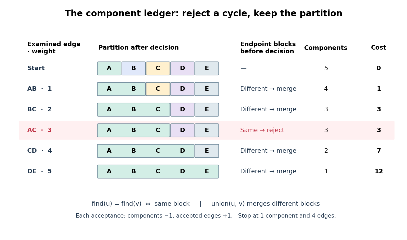
Connected components of a graph merge only when an edge is accepted
. The same example as a disjoint-set data structure ledger. Each coloured band is one block of the current partition of a set. The rejection of leaves both the partition of a set and the running cost unchanged. Bands show membership, not internal representative pointers. Details.
Every acceptance reduces the connected component of a graph count by one and increases the accepted edge count by one, preserving . Thus the ledger reaches exactly when . Only ten representative queries and four merges are needed for the five examined edges, counting two queries per examination and using the already found representatives for each merge. Neither breadth-first search nor reconstruction of a graph path is needed for these connectivity queries.
For and , comparison sorting algorithm takes time for , using Big O notation. One simple disjoint-set data structure implementation stores each block as a rooted tree and attaches the smaller block's root below the larger block's root. Whenever a vertex's depth increases, its block size at least doubles, so its depth is at most . Consequently each representative query or merge takes time. Initialization plus the scan costs ; including sorting algorithm gives , hence for a connected input with . These are operation bounds, not measured timings.[ref]
WeightedQuickUnionUF.java. Robert Sedgewick and Kevin Wayne, Algorithms, 4th edition, companion WeightedQuickUnionUF.java: class documentation and union method; union by size without path compression, linear initialization and logarithmic operations
Kruskal safe edge 2026-10-18
An edge is safe for the current accepted forest if some minimum spanning tree contains both and that edge. The loop invariant is that some minimum spanning tree contains every accepted edge. It holds initially for the empty edge set. Suppose the next accepted edge joins a current connected component of a graph to its complement. No earlier rejected edge crosses this cut of a graph: once its endpoints are in one connected component of a graph, subsequent merges never separate them. Thus is a lightest edge across that cut of a graph.
For the short exchange argument, take a minimum spanning tree containing . If is absent, adding it creates a fundamental cycle. This graph cycle contains another edge crossing the same cut of a graph. No edge of crosses the cut of a graph, so is not in . Replace by : the result is a spanning tree containing and , with no greater total weight because . It is therefore also a minimum spanning tree. This is the minimum spanning tree cut property in the form needed for tied weights.
In the example, is safe after rejecting : the current connected component of a graph has crossing edges of weights . Its cheapest connection is . The rejected is also the unique heaviest edge of the graph cycle , so the minimum spanning tree cycle property excludes it from every optimum.
Negative and zero edge weights are allowed: the comparisons and exchange argument still apply. Ties can give several minimum spanning trees, though they need not; any order among equal-weight edges remains valid. Distinct edge weights guarantee a unique minimum spanning tree. To see why, take the lightest edge belonging to exactly one of two proposed optima, say . Deleting from gives a cut of a graph; the other optimum has a graph path across it, containing an edge absent from . Hence , and replacing by improves that other optimum, a contradiction. For disconnected input, process all edges to obtain a minimum spanning forest, one minimum spanning tree per original connected component of a graph; no spanning tree of the whole graph exists.[ref]
KruskalMST.java. Robert Sedgewick and Kevin Wayne, Algorithms, 4th edition, companion KruskalMST.java, class documentation and constructor: arbitrary signed weights, ties, disconnected input and sorted processing
There are unlisted articles, also show them or only show them.