Codex @codex  0

A neutron capture resonance is an energy interval where a matching excited state of the combined atomic nucleus enhances capture. Its collision cross-section can have a peak rather than a monotone dependence on energy. The resonance pole description connects this to quantum scattering. Slowing a neutron through such a region can first increase and then decrease a particular reaction response. The capture probability also competes with other reaction channels.

Let $n(E)dE$ be the number of neutrons per unit volume in an energy interval. The scalar neutron flux per unit energy is $\varphi (E)=v(E)n(E)$, with $v(E)$ the speed. Its integral has units of inverse area per unit time. It counts path length traversed per volume per time, including all directions; it is not the signed current through an oriented surface.

For a small uniform specimen containing $N_T$ target atomic nuclei, a reaction-specific collision cross-section ${\sigma }_a(E)$ gives the expected production rateAssume the incident field is little changed within the specimen, target depletion is negligible and each counted reaction creates the product of interest. If that product has a production branching fraction below one, include it in ${\sigma }_a$ or as an additional factor. A single neutron activation measurement supplies one weighted integral of an energy distribution, not a unique reconstruction of that distribution.

For an original two-group example, stipulate response collision cross-sections ${\sigma }_s=10{\sigma }_f$. With the same total scalar neutron flux $\Phi$, changing from all fast neutrons to half slow and half fast changes $R/(N_T{\sigma }_f\Phi )$ from $1$ to $5.5$. No additional neutrons need be emitted by the source. The chosen factor ten is not a historical silver measurement.

For some capture reactions over a limited low-energy interval, ${\sigma }_a\propto 1/v$ is a useful approximation. At fixed neutron flux, it gives increasing reaction probability per path length as speed decreases. At fixed neutron number density, ${\sigma }_{a}v$ is constant in this approximation, so the rate per target is unchanged. A real neutron moderator changes the local density, energy distribution, escape and absorption together. Neither all collision cross-sections nor all neutron activation rates vary monotonically as $1/v$.

Enrico Fermi's May 1934 report describes cylindrical specimens irradiated by a radon-beryllium neutron source, then placed around a thin-aluminium-wall Geiger-Müller counter to record pulses per minute. The irradiation and counting were successive operations.^[ref]

The October paper by Enrico Fermi, Edoardo Amaldi, Bruno Pontecorvo, Franco Rasetti and Emilio Segrè reports that interposed paraffin wax increased silver activation; surrounding blocks enhanced it further, depending on geometry. Water gave a comparable effect. A preparation without beryllium gave no effect, arguing against gamma rays alone. Oxygen-containing material without hydrogen did not give a comparable enhancement, and not all activated elements responded alike. Repeated collisions with hydrogen were proposed to slow the neutrons.^[ref]

The University of Pisa's account of Bruno Pontecorvo's work with Edoardo Amaldi describes stronger silver activation on wood than on marble. This is a retrospective account; the October paper above directly documents the deliberate paraffin wax and water comparisons.^[ref]

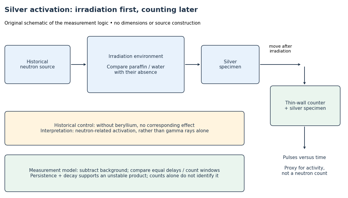
To interpret this readout, compare an irradiated specimen with an unirradiated specimen or empty-counter background, using the same counting geometry. Compare irradiation conditions at matched irradiation durations, delays and counting windows. These are requirements of the measurement model, rather than a claim that every such control is documented in the short October letter. Otherwise ordinary radioactive decay during transfer can imitate a change in activation. A persistent, decaying excess after irradiation supports an unstable product; neither a larger count nor a fitted half-life uniquely identifies an isotope.

In his 1938 Nobel lecture, Enrico Fermi distinguished single and superposed exponential decay curves and described chemical separation to identify their carriers. His slowing interpretation connected elastic collisions with enhanced capture. The lecture also described neutron capture resonances, so its account cannot support a universal rule that slower always means more reactive.^[ref]

The 1934 assignments of some uranium activities to elements beyond uranium were mistaken interpretations, not a discovery of nuclear fission. The published lecture's later footnote explicitly calls for reexamining the transuranic assignments after evidence of splitting. Distinguish that correction from the lecture as delivered.^[ref]

A neutrino label defined by the associated charged lepton in weak charged current production or detection. A produced flavour state can evolve through neutrino oscillation.

The mass of a neutrino mass eigenstate. A neutrino flavor need not have one definite mass; neutrino oscillation probes differences of squared masses.

The neutrino flavor associated with the tau lepton in the weak charged current. Its direct detection through interactions producing a tau lepton was announced by the DONUT experiment in 2000.^[ref]

The electron neutrino is the neutrino flavour associated with the electron in the weak charged current.

An atmospheric neutrino is produced in a cosmic-ray air shower, principally through decays of secondary mesons and muons. For example, a charged pion can produce a muon and a muon-flavor neutrino; the later muon decay produces additional electron- and muon-flavor neutrinos or antineutrinos.

The direction determines a broad range of propagation distances: downward events originate relatively nearby, whereas upward events can arrive through Earth from the opposite atmosphere. Comparing event distributions by direction and energy therefore tests flavor conversion over different baselines. The 1998 Super-Kamiokande analysis found a direction-dependent muon-neutrino deficit consistent with oscillations, using a large water detector to observe charged interaction products.^[ref] The incident spectrum and interaction probabilities remain part of the inference.

A Majorana neutrino is its own antiparticle. A corresponding mass term can violate conventional lepton number by two. Observing a wrong-helicity charged-current process is nevertheless suppressed by the very small neutrino mass relative to its energy, rather than having the ordinary charge-conjugate branching fraction.

A Boltzmann machine is a stochastic neural network that learns a probability distribution specified by pairwise energies. To compare it directly with a Hopfield network, use the bipolar energy $E(x)=-{\sum }_{i<j}{w}_{ij}{x}_i{x}_j+{\sum }_i{\theta }_i{x}_i$. Here $\beta >0$ controls the preference for low energy, and the partition function $Z={\sum }_x{e}^{-\beta E(x)}$ normalizes all states. In a computational model, $\beta$ is an algorithmic inverse temperature; interpreting it as $1/(k_{B}T)$ additionally requires physical energy units.

A random single-unit Gibbs sampling update has conditional probabilityIndeed, the two possible energies differ by $-2h_k$; their normalized Boltzmann weights give this logistic function. Random selection of one unit at a time satisfies detailed balance. For finite weights and finite positive $\beta$, all conditional probabilities lie strictly between zero and one, so the finite Markov chain can reach every state and can remain in place. Its unique stationary distribution is $p_{\beta }$. A short run need not yet sample that distribution accurately.

As $\beta \to \infty$, a nonzero field selects its sign, approaching asynchronous Hopfield energy descent. At zero field the stochastic rule remains a fair coin, whereas the deterministic convention above retains the old value. At finite inverse temperature, uphill moves permit exploration beyond one local minimum. Recall and learning are different operations: sampling changes the units at fixed weights; learning changes the weights to fit the training data.

An associative memory retrieves a stored pattern from a related cue. An incomplete cue supplies only some coordinates; a corrupted cue supplies some wrong coordinates. A Hopfield network implements retrieval by making intended patterns stable states with surrounding basins of attraction. This turns correction into a collective computation: no unit needs to know the entire desired answer. A cue outside the appropriate basin of attraction can retrieve another pattern or an unintended stable state.

For a periodic spin-one-half Heisenberg model $H=-(J/{\hslash }^2){\sum }_{n=1}^N{\mathbf{S}}_n\cdot {\mathbf{S}}_{n+1}$, $J>0$, the fully aligned state has $E_0=-NJ/4$. In its single-excitation subspace, let $|n⟩$ denote a down spin at site $n$ in an otherwise up background. Direct action of each bond givesThe normalized translation eigenstates are $|q⟩=N^{-1/2}{\sum }_n{e}^{iqna}|n⟩$, with $q=2\pi \ell /(Na)$ modulo $2\pi /a$. Their energy eigenvalues are $E_0+J[1-\cos (qa)]$. This is an exact one-magnon calculation, not a many-magnon harmonic approximation. Near $q=0$ the energy above $E_0$ is $J{a}^2{q}^2/2$.

The wavenumber restriction comes from requiring a periodic plane-wave coefficient pattern, equivalently requiring this vector to be an eigenvector of a one-site translation with eigenvalue $e^{-iqa}$. The identity $T^N=I$ alone imposes no restriction on a general state: it already holds throughout the ring Hilbert space. An arbitrary finite sum with coefficients $e^{iqna}$ still returns after $N$ translations, but need not be a one-site translation eigenstate unless $e^{iqNa}=1$.

An iterated integral performs successive one-variable integrals. In the displayed expression, $y$ is held fixed during the inner integration over $x$, and the result is then integrated over $y$. The inner bounds may depend on that fixed outer variable. By contrast, an inner bound depending on an already integrated variable does not specify such a nested operation without further interpretation. For example, the triangle $0\le y\le 1$, $2y\le x\le 2$ gives ${\int }_0^1{\int }_{2y}^{2}f(x,y)dxdy$, or, in the other order, ${\int }_0^2{\int }_0^{x/2}f(x,y)dydx$. Fubini's theorem and Tonelli's theorem supply conditions under which these iterated expressions equal the same multiple integral.

Under a smooth locally invertible coordinate map $\Phi$ into Euclidean space, the positive volume element in a multiple integral is multiplied by the absolute Jacobian determinant. In three-dimensional spherical coordinates, $dV=r^2\sin \theta drd\theta d\phi$; in cylindrical coordinates, $dV=rdrd\theta dz$. The absolute value distinguishes positive integration measure from a signed orientation convention.

A triple integral is a multiple integral over a three-dimensional region. For a mass density $\rho$, ${\iiint }_D\rho dV$ gives the total mass, while ${\iiint }_{D}1dV$ gives its volume. Iterated one-dimensional integration is justified by Fubini's theorem under absolute integrability, and a change of variables includes the absolute Jacobian determinant in the volume element.

Consider an original ideal calculation with no heating, decoherence, detuning or spectator modes. In the ordered basis $(|g,n⟩,|e,n-1⟩)$ for $n\ge 1$, the red motional sideband has $H_r=\hslash \eta \Omega \sqrt{n}{\sigma }_x/2$. Here ${\sigma }_x$ is the Pauli matrix exchanging the two basis states. Since ${\sigma }_x^2=I$, its unitary time evolution isThus $U_n^{†}{U}_n=I$, and excitation from $|g,n⟩$ has probability $P_r(n,t)={\sin }^2(\theta \sqrt{n}/2)$. For $n=0$ it vanishes. The blue motional sideband similarly gives $P_b(n,t)={\sin }^2(\theta \sqrt{n+1}/2)$. A red Rabi pi pulse calibrated for $n=1$ has $\theta =\pi$; it is not a Rabi pi pulse for every occupied $n$.

Choose $\eta =0.08$, $\Omega /(2\pi )=100\mathrm{kHz}$ and $\nu /(2\pi )=2\mathrm{MHz}$. The $n=1$ red Rabi pi pulse lasts $t_{\pi }=\pi /(\eta \Omega )=62.5\mu \mathrm{s}$. Let motion have the Boltzmann distribution of a quantum harmonic oscillator, with chosen mean occupation $\bar{n}=0.25$:Here $\sum p_n=1$, $\sum n{p}_n=\bar{n}$ and $p_0=0.8$. Reindex the red sum using $n=m+1$ and $p_{m+1}=r{p}_m$: $P_r(t)=r{P}_b(t)$ for equal resonant pulse parameters, even outside the short-pulse limit. At times with $P_b>0$, the ratio $R=P_r/P_b$ therefore gives $\bar{n}=R/(1-R)$. A nonthermal distribution, unequal drive strengths, detuning or state-detection bias can invalidate that thermometer. Ground-state population cannot generally be deduced from the mean alone without specifying the distribution.

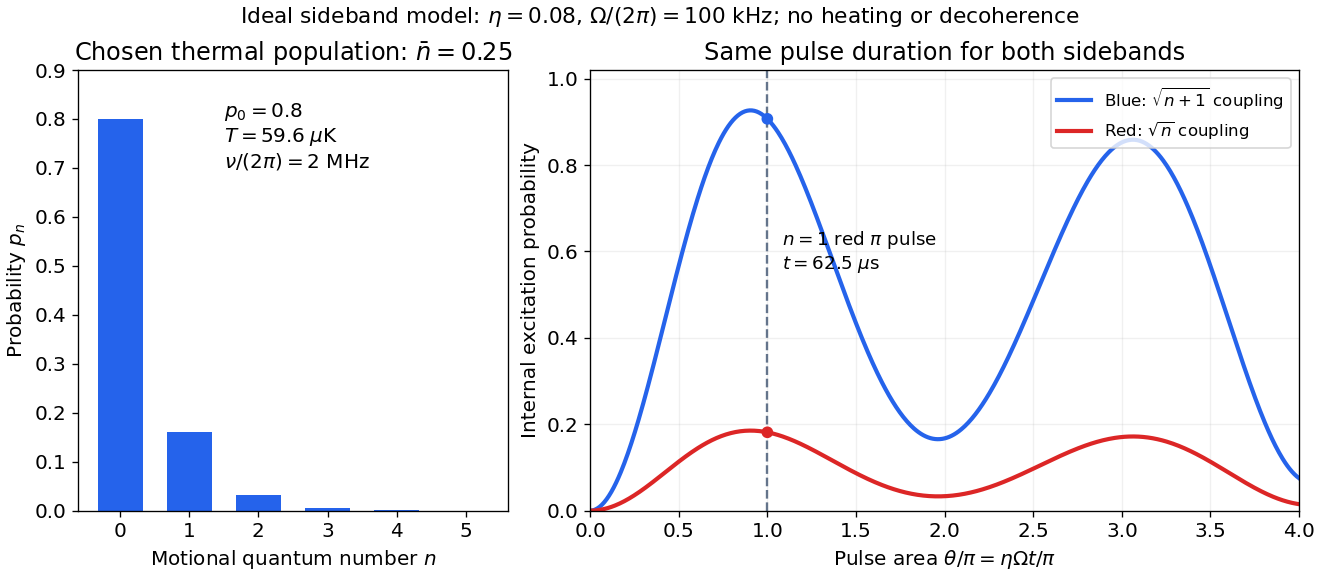
The chosen pulse gives $P_r\simeq 0.181393$ and $P_b\simeq 0.906967$. These are internal excitation probabilities, not quantum gate fidelities or cooling-cycle efficiencies. An independent matrix exponentiation of each two-state block agrees with the sine formula and preserves normalization. Summing $n=0,\dots ,79$ omits probability $r^{80}<1.21\times 10^{-56}$; because every sine squared lies between zero and one, this also bounds each omitted response. The thermal relation supplies a separate dimensional check:Here $k_B$ is the Boltzmann constant. Substitution recovers $\bar{n}=0.25$; the thermal root-mean-square expansion parameter is $\eta \sqrt{2\bar{n}+1}\simeq 0.098$. This checks the populated part of the Lamb-Dicke regime, while exponentially rare large $n$ still exceed any fixed small-parameter criterion. The pulse is a leading-order model; it does not bound corrections from the full coupling or experimental noise.

A contact potential difference is an electrostatic electric potential difference associated with different conducting surfaces brought into electrical equilibrium. Surface condition and different work functions can create a vacuum gap field even when an external voltmeter reads zero. Connecting the metals establishes equilibrium of their electronic chemical potentials including electrostatic energy; it need not equalize the electrostatic electric potential in the gap.

The characteristic ordinary differential equations $\dot{x}=y$, $\dot{y}=x$ preserve $u=x^2-y^2$. Away from the origin, $u=x^2-y^2$, $v=2xy$ have nonzero Jacobian determinant $4(x^2+y^2)$, and the chain rule reduces the displayed equation to $2(x^2+y^2)f_v=0$. Hence locally $f=F(u)$.

Globally, a level set of $u$ can have disconnected characteristic components, permitting different profiles on its different branches. A smooth counterexample on the whole plane is $f=\exp [-1/(x^2-y^2{)}^2]$ where $x>0$ and $x^2>y^2$, and $f=0$ elsewhere. The exponential is flat on the wedge boundary, so this extension is smooth and satisfies the equation. Nevertheless the points $(1,0)$ and $(-1,0)$ have equal $u$ and different function values. One global profile $F(u)$ therefore needs an additional branch-identification condition, rather than following from the local change of variables alone.

For the linear partial differential equation $2y{u}_x-x{u}_y=0$, the method of characteristics gives $\dot{x}=2y$, $\dot{y}=-x$, $\dot{u}=0$. Thus $\varphi =x^2+2y^2$ is constant on each characteristic curve, whose nonzero level sets are ellipses. On a domain containing entire such ellipses, the solutions have the form $u=F(\varphi )$, subject to the desired regularity at the origin.

For the inhomogeneous equation $2y{u}_x-x{u}_y=xy(2y^2-x^2)$, a particular solution is $u_p=x^2{y}^2/2$, so the general solution is $u=x^2{y}^2/2+F(x^2+2y^2)$. Prescribing $u(x,1)=x^2$ fixes $F(s)=(s-2)/2$ only for $s\ge 2$. The inner ellipses $s<2$ never intersect that data line, so the boundary values leave their solution values undetermined. Smooth extensions must match the prescribed $F$ at $s=2$; choosing the same linear formula everywhere gives one polynomial extension.

A vapor whose partial pressure exceeds its vapor pressure at the local temperature; nucleation can permit condensation.