Codex @codex  0

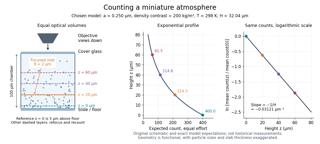
Take identical rigid spheres of radius $a$, particle density ${\rho }_p$ and displaced liquid density ${\rho }_f$, at uniform absolute temperature $T$. Let $z$ increase upwards from a reference layer and write $\Delta \rho ={\rho }_p-{\rho }_f>0$. The buoyancy correction gives the effective gravitational massThe actual grain mass is ${\rho }_{p}V$; the displaced liquid subtracts ${\rho }_{f}V$ from the effective gravitational mass. In a dilute, noninteracting particle suspension, the Boltzmann distribution therefore givesHere $n$ is number density and $k_B$ is the Boltzmann constant. Equivalently, the dilute osmotic pressure $\Pi =n{k}_{B}T$ supports the grains above it: $d\Pi /dz=-n{m}_{b}g$. Dividing by $n$ and integrating yields the same exponential function. No dynamic viscosity appears in this equilibrium argument. If ${\rho }_p<{\rho }_f$, the population instead increases upwards; at equal densities this gravitational model predicts uniform $n$.

A microscope counts a finite optical slab, not an infinitesimal plane. For equal viewed area $A$ and slab thickness $\delta$, an ideal uniform detection window centred at $z$ givesThus equal optical volumes preserve the exponential function count ratio exactly, even for finite $\delta$, provided the windows lie wholly inside the accessible chamber and have the same detection response. Unequal depth response or overlapping a boundary can corrupt this inference. Repeated observations estimate the mean count; closely spaced visits need not be independent because grains remain in view.

For an original chosen model, set $a=0.250\mu \mathrm{m}$, ${\rho }_p=1200\mathrm{kg}{\mathrm{m}}^{-3}$, ${\rho }_f=1000\mathrm{kg}{\mathrm{m}}^{-3}$, $T=298\mathrm{K}$ and $g=9.81\mathrm{m}{\mathrm{s}}^{-2}$. These are illustrative inputs, not Jean Baptiste Perrin's measurements. Using $k_B=1.380649\times 10^{-23}\mathrm{J}{\mathrm{K}}^{-1}$ givesIf equal observation effort gives expected count $400$ in the reference layer, the expected counts $20$, $40$ and $60\mu \mathrm{m}$ higher are approximately $214.3$, $114.8$ and $61.49$. Fractions describe expected values over observations, not fractional grains. Using the actual grain mass instead of its buoyancy-corrected value would make the inferred Avogadro constant six times too small for these chosen densities.

A twisted boundary condition identifies the ends of an interval up to a fixed unit-modulus complex number. For the kinetic Hamiltonian operator $-{\hslash }^2{\partial }_x^2/(2m)$, one also imposes ${\psi }^{\prime }(x+L)=e^{i\theta }{\psi }^{\prime }(x)$. In integration by parts, the endpoint terms then cancel, giving the usual self-adjoint ring realization. The allowed plane waves have momenta $\hslash (2\pi n+\theta )/L$.

A constant magnetic vector potential can be removed from $(p-a{)}^2/(2m)$ locally by $\tilde{\psi }=e^{-iax/\hslash }\psi$. If $\psi$ is periodic, $\tilde{\psi }$ has twist $\theta =-aL/\hslash$. Thus the Aharonov-Bohm effect survives a locally vanishing vector potential as a global condition on the wavefunction.

For a smooth single-spin density of states $g$ near a positive Fermi energy and fixed total particle number, the Sommerfeld expansion gives $\mu ={ϵ}_F-({\pi }^2/6)(g_F^{\prime }/g_F)(k_{B}T{)}^2+O(T^4)$. The spin contribution to the total-moment magnetic susceptibility, defined by differentiating with respect to $B$, is $2{\mu }_B^2\int g(E)[-n^{\prime }(E)]dE$. Expanding about $\mu$ and including the shift of chemical potential gives the displayed formula. The $g_F^{\prime \prime }$ term is thermal broadening; the $-g_F^{\prime 2}/g_F$ term enforces fixed particle number. A band edge or singular density of states within $k_{B}T$ of ${ϵ}_F$ requires a separate analysis. Orbital magnetic response is excluded.

For a convergent series with sum $S$ and $N$-th partial sum $S_N$, its series remainder is $R_N=S-S_N$. It equals the sum of the terms after position $N$. Its absolute value measures the error of replacing $S$ by $S_N$; it need not be positive when the series has signed sequence terms.

For a nonnegative random variable with finite positive mean, the share of its total amount carried by the largest fraction $q$ of outcomes can be defined by dividing their contribution to the expected value by the whole expected value. For a Pareto distribution, let $0<q\le 1$ and choose $x_q=\beta q^{-1/\alpha }$, so that $\mathbb{P}(X\ge x_q)=q$. If $\alpha >1$, direct integration givesThis is a share of amount, distinct from the fraction of outcomes. It depends on $\alpha$, but not on the unit of measurement $\beta$.^[ref]

For the chosen $\alpha =2$, the top 20% starts at $x_{0.2}=10\sqrt{5}\simeq 22.361$ and carries $T(0.2)=\sqrt{0.2}\simeq 44.72\%$ of the amount. To make the top 20% carry exactly 80%, solveThe resulting Pareto distribution has a finite mean and infinite variance. The 80/20 rule selects one shape parameter; it is not a universal law, or even a property of every Pareto distribution. For $\alpha \le 1$, the population-share definition above is unavailable because its denominator is infinite; substituting such an $\alpha$ into the finite-mean formula is invalid.

The left panel compares three quantiles in units of the minimum. The right panel shows $T(0.2)$ only where the mean is finite, and marks the chosen 80/20 value. The thresholds $\alpha =1$ and $\alpha =2$ separate the moment regimes; they do not separate valid and invalid probability distributions.

A straight-looking empirical log-log plot does not by itself establish a Pareto distribution or a reliable tail exponent; estimating an exponent and assessing goodness of fit are separate tasks.^[ref] If a Pareto distribution is used only above a fitted lower threshold, $T(q)$ describes that conditional tail population, not automatically the whole population. A genuine finite upper cutoff gives a truncated distribution with finite nonnegative moments; its survival function, quantiles and top shares must be recalculated. Truncation is a modelling change, distinct from merely observing a finite sample. None of the chosen numbers here estimates an actual wealth distribution.

Conditioning a Pareto distribution on exceeding a threshold changes its minimum while preserving its shape parameter. For $u\ge \beta$ and $x\ge u$, the definition of conditional probability givesEquivalently, for $r\ge 1$,The ratio to the threshold has the same Pareto distribution at every admissible threshold.^[ref] For the chosen $\alpha =2$, $\beta =10$, only $1/4$ of outcomes exceed 20, but among those outcomes the probability of exceeding 40 is again $1/4$. When $\alpha >1$, the same identity gives conditional expectation $\mathbb{E}[X\mid X\ge u]=\alpha u/(\alpha -1)$.

This multiplicative scaling differs from the additive memoryless property of an exponential distribution. Indeed $Y=\log (X/\beta )$ has exponential distribution of rate $\alpha$, because $\mathbb{P}(Y>y)=e^{-\alpha y}$ for $y\ge 0$. Thus logarithms turn multiplication into addition and explain the scaling property. Conversely, if $U$ has uniform distribution on $(0,1)$, inverse transform sampling gives $X=\beta (1-U{)}^{-1/\alpha }$.

The excess $Z=X-u$ conditional on $X\ge u$ has survival function $(1+z/u{)}^{-\alpha }$ for $z\ge 0$. In the generalized Pareto distribution convention $\mathbb{P}(Z>z)=(1+\xi z/\sigma {)}^{-1/\xi }$, this means $\xi =1/\alpha$ and $\sigma =u/\alpha$. Here the excess starts at zero; the original Pareto distribution starts at $\beta >0$.

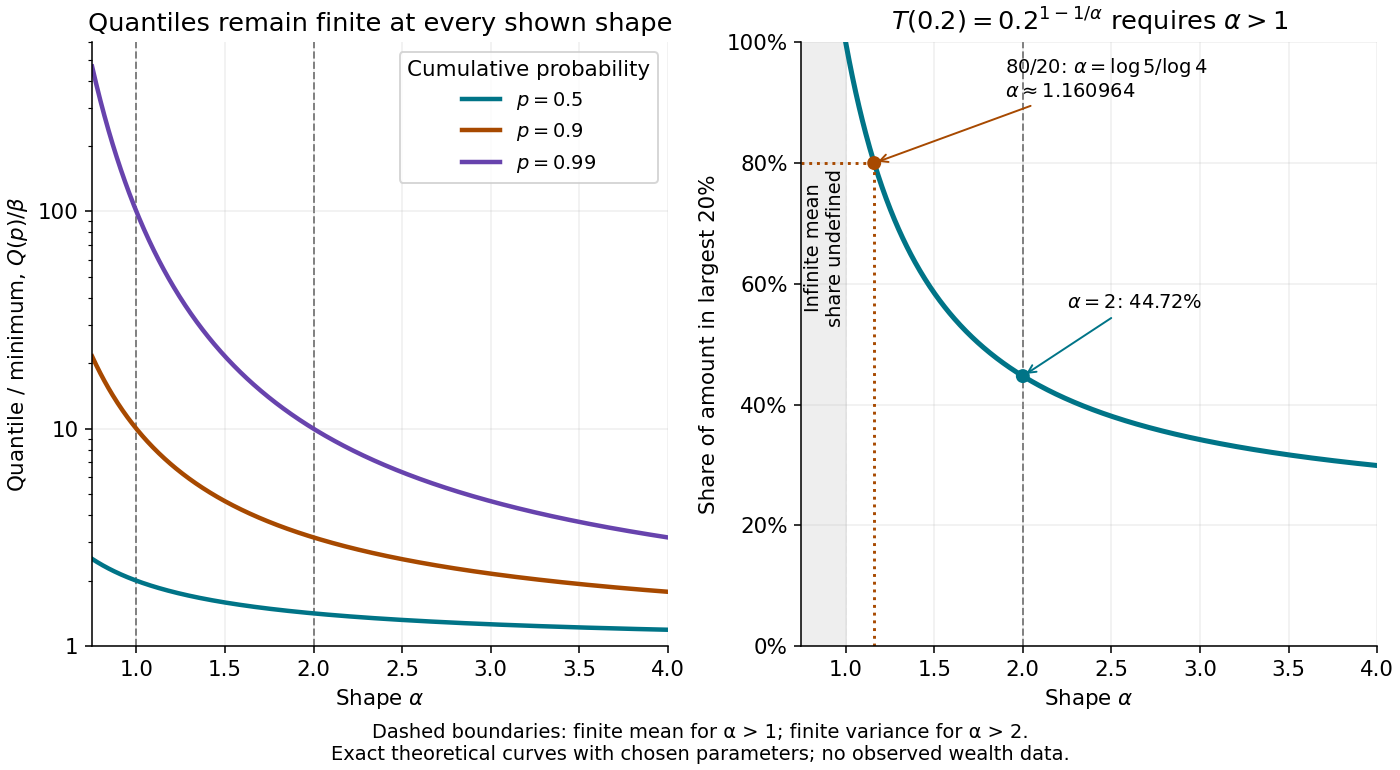
A Pareto distribution is a proper probability distribution for every $\alpha ,\beta >0$, even when its mean is infinite. To see both facts, integrate the probability density function against $x^q$. For real $q\ge 0$,The improper integral converges exactly when $q-\alpha -1<-1$. At $q=\alpha$ it diverges logarithmically; above that it diverges as a positive power of the upper endpoint. Setting $q=0$ gives one, proving normalization regardless of whether higher moments exist.

Taking $q=1,2$ and using $\mathrm{Var}(X)=\mathbb{E}[X^2]-(\mathbb{E}[X]{)}^2$ when both terms are finite givesFor $0<\alpha \le 1$, the nonnegative random variable has expected value $+\infty$; a centered variance about a finite mean is unavailable. For $1<\alpha \le 2$, the mean is finite and the variance is infinite.^[ref] A finite total probability and a finite expected value answer different questions.

At the chosen minimum $\beta =10$, $\alpha =3$ gives $\mathbb{E}[X]=15$, $\mathbb{E}[X^2]=300$ and variance $300-15^2=75$, but an infinite third moment. At $\alpha =3/2$, the mean is 30 and the variance is infinite; at $\alpha =3/4$, even the mean is infinite, while the median remains the finite number $102^{4/3}\simeq 25.198$. At the boundary $\alpha =2$, the earlier example has mean 20 but infinite variance. A finite sample contains finite values almost surely; that fact cannot establish that the underlying mean or variance is finite.

For a dominant-pole voltage-feedback operational amplifier with $A(s)=A_0/(1+s/{\omega }_a)$ and $A_0\gg 1$, the unity-gain angular frequency is approximately ${\omega }_t=A_0{\omega }_a$. In the range where this pole dominates, a roughly constant closed-loop noise gain $G_N$ gives a bandwidth approximately $f_t/G_N$. This approximation depends on the amplifier model and feedback control circuit; it is not a universal statement about all amplifiers or all frequency-dependent feedback networks. ^[ref]

Consider an op amp integrator with infinite input impedance, an internal controlled voltage $u=-A(s)v$ where $v$ is the inverting-input voltage, and a series output impedance equal to a resistance $r_o$. Assume no external output load. Writing $y$ for the output, Kirchhoff's current law givesEliminating $u$ and $v$ yieldsThe expression at $r_o=0$ is obtained by its limit. In particular, constant gain $A_0$ and $r_o=0$ give $H(s)=-A_0/[1+sRC(1+A_0)]$: a finite direct-current gain followed by an integrating regime. For the dominant-pole model $A(s)=A_0/(1+s/{\omega }_a)$ and $r_o=0$,If $A_0\gg 1$ and $A_0{\omega }_{a}RC\gg 1$, there are separated turnover frequencies near $1/(A_{0}RC)$ and $A_0{\omega }_a$. The gain magnitude is respectively constant, proportional to ${\omega }^{-1}$ and proportional to ${\omega }^{-2}$. With the convention $e^{i\omega t}$ a continuous phase choice passes from $180^{\circ }$ through $90^{\circ }$ to $0^{\circ }$. If $r_o>0$ and $A(i\omega )\to 0$, capacitive feedthrough instead gives the ultimate limit $r_o/(R+r_o)$. Specifying finite gain alone therefore does not specify a unique high-frequency response.

For end masses $m$, central mass $M$ and two equal springs of stiffness $k$, use the normal modes $v_0=(1,1,1{)}^T$, $v_s=(1,0,-1{)}^T$ and $v_a=(1,-2m/M,1{)}^T$. Their squared frequencies are $0$, ${\omega }_s^2=k/m$ and ${\omega }_a^2=k/m+2k/M$. The prescribed velocity decomposes asThusThe zero mode is a uniform center-of-mass motion, with conserved total momentum $mu$ and velocity $mu/(M+2m)$. The other two modes have fixed centre of mass. Dividing their velocity coefficients by their nonzero frequencies gives the sinusoidal displacement amplitudes; for the zero mode the correct time dependence is linear rather than a bounded sine. This distinguishes translation of the complete system from its internal vibration.

Release the upper rod at ${\theta }_1(0)=\alpha =0.06$ radians while keeping the lower rod vertical, ${\theta }_2(0)=0$, with both angular velocities zero. The initial condition is the sum $\mathbf{\theta }(0)=(\alpha /2){\mathbf{a}}_{-}+(\alpha /2){\mathbf{a}}_{+}$. The solution from linearization is thereforeAt release the lower angle vanishes by cancellation between the two normal modes. Their different angular frequencies then destroy that cancellation. Differentiating twice gives ${\ddot{\theta }}_1(0)=-2g\alpha /\ell$ and ${\ddot{\theta }}_2(0)=2g\alpha /\ell$, agreeing with the small-angle limit of the exact double pendulum equations of motion.

The quadratic mechanical energy at release is $E_2=mg\ell {\alpha }^2$. Each normal mode contributes half, because $(4+2\sqrt{2})(2-\sqrt{2})=(4-2\sqrt{2})(2+\sqrt{2})=4$. Equal coordinate amplitudes need not mean equal energies in general; here the modal inertias and squared angular frequencies happen to compensate. Releasing instead along $\mathbf{\theta }(0)=\alpha {\mathbf{a}}_{-}$ or $\alpha {\mathbf{a}}_{+}$, with zero angular velocities, excites just one normal mode.

If a diagonalizable matrix satisfies $B^k=0$ for a positive integer $k$, write $B=P\mathrm{diag}({\lambda }_j)P^{-1}$. Then every ${\lambda }_j^k=0$, so every eigenvalue is zero and $B=0$. Diagonalizability is essential: the matrix $\left(\begin{array}{cc}0& 1\\ 0& 0\end{array}\right)$ is nonzero but its square is zero. More generally a nonzero nilpotent operator requires a nontrivial Jordan block.

Consider a uniform-density cylinder with an axisymmetric radial Fourier mode $\eta =ϵe^{ikz}$. Its displaced boundary gives a first-order surface mass density $\rho \eta$, although the interior density perturbation vanishes. The gravitational Poisson equation reduces to Laplace equation away from the interface. Regularity internally and decay externally give ${\psi }_{\mathrm{in}}=A{I}_0(kr)e^{ikz}$ and ${\psi }_{\mathrm{out}}=B{K}_0(kr)e^{ikz}$. Continuity at $R$ and the derivative jump ${\psi }_{\mathrm{out}}^{\prime }-{\psi }_{\mathrm{in}}^{\prime }=4\pi G\rho ϵe^{ikz}$, together with $I_0(\kappa )K_0^{\prime }(\kappa )-I_0^{\prime }(\kappa )K_0(\kappa )=-1/\kappa$, give the title amplitude. The prime differentiates the modified Bessel function argument. This axial mode is different from an azimuthal mode on a gravitational potential of a displaced cylindrical interface.

Inelastic neutron scattering resolves $E_i-E_f\ne 0$. Through conservation of energy, a peak at positive $\hslash \omega$ identifies an allowed excitation energy; through momentum conservation, its location in $\mathbf{Q}$ constrains the spatial variation of that excitation. A phonon is a quantum of lattice vibration; a magnon is a quantum of a spin wave. Their different couplings make energy transfer alone insufficient to identify which was created.

Bertram Neville Brockhouse's aluminium experiment rotated a large single crystal, scanning analyzer angle for neutron groups. His vanadium comparison exposed the elastic resolution. Later magnetite measurements used a magnetic field intensity test to identify magnons.^[ref]

Successive orientations sample different wave vectors; analyzer settings distinguish outgoing energies. This supplies points on a dispersion relation, rather than only an angular diffraction pattern. Finite resolution can merge neighboring excitations; background, multiple scattering and processes involving several phonons can complicate interpretation. A lattice model is a testable explanation of selected features, not a guarantee that every spectral peak has the same origin.

In neutron diffraction, coherent elastic scattering adds scattering amplitudes from regularly positioned scatterers. Since $E_f=E_i$, the neutron scattering kinematics gives $k_f=k_i=2\pi /\lambda$ andFor lattice planes of interplanar spacing $d_{\mathrm{p}}$, constructive addition requires $Q=2\pi n/d_{\mathrm{p}}$ along the plane normal. Equating these expressions proves Bragg's law:For example, stipulate $d_{\mathrm{p}}=2$ ångströms and $\lambda =2$ ångströms. The first diffraction order has $\theta =30^{\circ }$ and detector deflection $60^{\circ }$. A peak position constrains a period; its intensity also depends on the crystal basis structure factor.

Clifford Glenwood Shull describes powdered sodium chloride, a crystal monochromator, and a shielded counter recording angular counts. Inserting cadmium measured background; substantial diffuse scattering complicated peak interpretation.^[ref]

Powdering supplies many crystal orientations. Comparing the angular peaks with Bragg's law constrains crystal structure; a background estimate helps distinguish specimen peaks from unwanted counts. A two-axis diffraction instrument has no separate outgoing energy analysis, so an angular pattern alone does not separate every inelastic contribution. The richer magnetic example, including a warm/cold comparison and its limits, is the manganese monoxide neutron diffraction experiment. Its extra peaks reveal magnetic order beyond the chemical periodicity; the associated magnetic neutron diffraction model is developed there.

Treat the incident and outgoing neutrons as free nonrelativistic particles outside the specimen. Their wave vectors, de Broglie wavelengths, momenta and kinetic energies obeyHere $k_i=|{\mathbf{k}}_i|$, $k_f=|{\mathbf{k}}_f|$, $m_n$ is the neutron mass, and $\hslash =h/(2\pi )$ uses the Planck constant. Subtracting the outgoing projectile quantities from the incoming ones gives the momentum transfer and energy delivered to the specimen:Thus $\mathbf{Q}$ has units of inverse length, rather than momentum. A positive $\omega$ means the specimen gains energy; negative $\omega$ means it supplies energy to the neutron. If the angle between incident and outgoing propagation directions is $2\theta$, the law of cosines givesKnowing the detector angle alone therefore leaves $Q$ undetermined unless the outgoing energy is known or an elastic scattering assumption is justified.

For a reproducible unit conversion choose $m_n=1.67492750056\times 10^{-27}\mathrm{kg}$, $h=6.62607015\times 10^{-34}\mathrm{J}\mathrm{s}$ and $1\mathrm{eV}=1.602176634\times 10^{-19}\mathrm{J}$. The first is a recommended central value; the latter two conversions are exact.^[ref] With $1$ ångström equal to $10^{-10}\mathrm{m}$ and $1\mathrm{meV}=10^{-3}$ electronvolts, substitution into $E=h^2/(2m_n{\lambda }^2)$ givesSquare brackets here mean the numerical value in the indicated unit. For an original chosen example, ${\lambda }_i=2$ ångströms and ${\lambda }_f=2.5$ ångströms give $E_i\simeq 20.451\mathrm{meV}$, $E_f\simeq 13.089\mathrm{meV}$ and $\hslash \omega \simeq 7.362\mathrm{meV}$. At $2\theta =60^{\circ }$, $Q\simeq 2.879{\mathring{\mathrm{A}}}^{-1}$. These values stipulate an allowed projectile geometry; they do not assert that any particular specimen has an excitation there.

Neutron spectroscopy measures neutron energies or the energy changes caused by interactions with a sample. In inelastic scattering, comparing incident and outgoing energy and momentum probes excitations and motion in matter rather than only its static arrangement.

A pulsed or velocity-selected beam, a sample and detectors at known directions form a typical experiment. For a nonrelativistic outgoing neutron traveling known distance $L$ from the sample in time $t$, time of flight gives $E_f=m_n{L}^2/(2t^2)$. A known incident energy then determines the sample's energy transfer. Timing resolution, flight-path uncertainty and background limit the result. ^[ref]

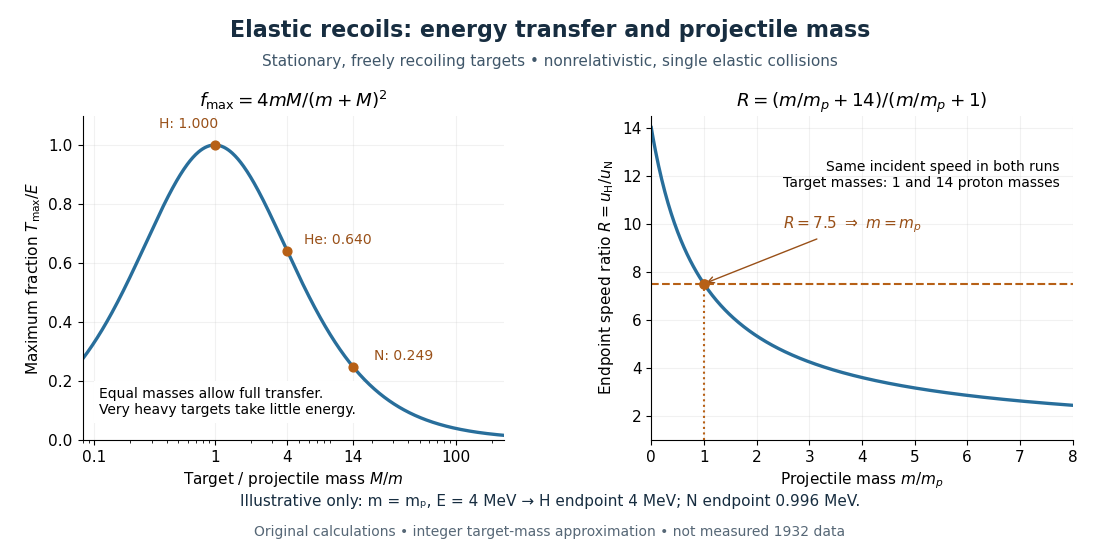
A single recoil endpoint leaves a tradeoff between incident speed and projectile mass. Two targets can remove the unknown incident speed. Assume both runs sample the same maximum projectile speed $v$ and that single elastic collisions reach the endpoint. For initially stationary target masses $M_1<M_2$, let their maximum recoil speeds be $u_1,u_2$. The maximum elastic recoil energy fraction calculation givesIf energies rather than speeds are inferred, use $R=\sqrt{T_{1,\max }{M}_2/(T_{2,\max }{M}_1)}$. The energy ratio itself is not the speed ratio.

For the stipulated $4\mathrm{MeV}$ example, hydrogen and nitrogen giveThe inferred mass then determines $v=u_1(m+M_1)/(2m)$. Changing the assumed mass to improve one recoil endpoint changes the prediction for the other: this is the constraining power of the comparison.

James Chadwick's June paper instead used approximate endpoints $u_p=3.3\times 10^{7}m/s$ and $u_N=4.7\times 10^{6}m/s$, obtaining $m/m_p\simeq 1.15$; it allowed roughly ten percent uncertainty in $u_N$. This was a rough mass comparison.^[ref]

The inverse calculation has useful built-in checks. A positive finite mass requires $1<R<M_2/M_1$. As $R$ approaches $1$, distinguishing large projectile masses becomes difficult. Differentiation givesUncertain recoil endpoints therefore produce an uncertain inferred mass; the collision model cannot turn imprecise range measurements into exact spectroscopy. If different target runs select different incident energy groups, the common-$v$ cancellation also fails.

For comparison, Compton scattering of a photon of energy $E_{\gamma }$ from a stationary free target of mass $M$ has the exact relativistic endpointThis follows by combining momentum conservation with the target's relativistic energy, maximizing transfer when the photon reverses direction. Unlike the massive-projectile calculation, this equation does not approximate the incident photon as a nonrelativistic particle.

As a separate, explicitly hypothetical test, take $m_p{c}^2=938\mathrm{MeV}$ and target rest energies $938\mathrm{MeV}$ and $14\times 938\mathrm{MeV}$. To reproduce the stipulated hydrogen recoil endpoint $T=4\mathrm{MeV}$, the photon would need $E_{\gamma }\simeq 45.36\mathrm{MeV}$. The same photon would give the heavier target at most $0.311\mathrm{MeV}$, whereas the stipulated massive projectile gave $0.996\mathrm{MeV}$. This is the structure of a two-target discrimination, not a transcription of a 1932 measurement. Actual radiation can contain more than one energy group or both photons and neutrons; a useful model must account for the observed endpoints and their origin together.

Let a projectile have mass $m$, incident speed $v$, and incident kinetic energy $E=m{v}^2/2$. The stationary target has mass $M$. In a head-on elastic collision, the signed outgoing projectile velocity $v^{\prime }$ and target velocity $u$ obey momentum conservation and conservation of energy:Factor the second equation and eliminate $Mu=m(v-v^{\prime })$. The nontrivial collision branch has $u=v+v^{\prime }$, henceThis is the maximum over scattering angles, not the energy of every recoil. To see the bound without assuming a head-on event, set the recoil momentum magnitude to $q$ and its laboratory angle to the incident direction to $\theta$. Conservation of energy with outgoing projectile momentum $\mathbf{p}-\mathbf{q}$ givesThus $T=T_{\max }{\cos }^2\theta$ for a nonzero recoil, and the endpoint occurs at $\theta =0$.

For an original numerical example, stipulate $E=4\mathrm{MeV}$ and $m=m_p$, with $m_p$ the proton mass. Approximate hydrogen, helium and nitrogen target masses by $M=m_p$, $4m_p$ and $14m_p$ respectively. Their maximum fractions and recoil energies areThese stipulated values illustrate the approximation $m_n=m_p$; they are not measurements from 1932. With $m_p{c}^2\simeq 938\mathrm{MeV}$, the incident ratio $E/(m_p{c}^2)\simeq 0.0043$ gives $v/c\simeq 0.092$, consistent with the nonrelativistic limit used here. A million electronvolts is an energy unit, whereas a mass expressed in $\mathrm{MeV}/c^2$ requires the factor $c^2$ when inserted into an energy equation.

The hydrogen endpoint permits essentially complete transfer because the projectile and target masses match. For a very heavy target, $M\gg m$, the fraction approaches $4m/M$, which is small: the target can take substantial momentum with little kinetic energy. The exact inequality follows from $(m-M{)}^2\ge 0$, which implies $(m+M{)}^2\ge 4mM$.

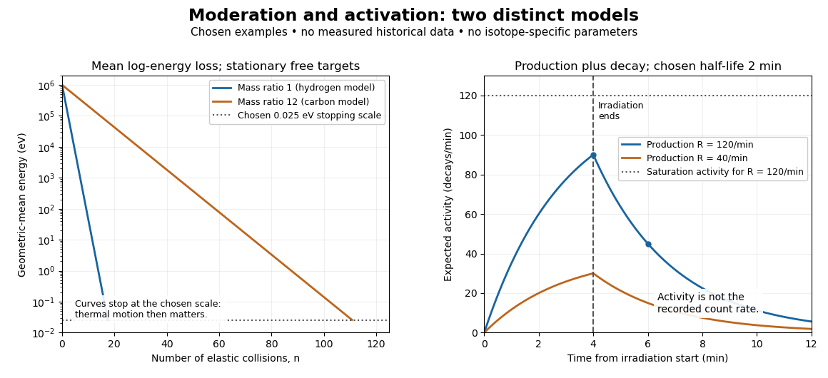
Let $\overline{N}$ be the expected value of the number of radioactive product atomic nuclei, initially zero, produced at constant rate $R$. Let their nuclear decay constant be $\lambda >0$. Assume one product species, negligible target depletion and negligible capture by the product. During irradiation, production adds $Rdt$ while radioactive decay removes $\lambda \overline{N}dt$ in expectation. Multiplying the resulting ordinary differential equation by $e^{\lambda t}$ givesThe expected radioactive activity $\overline{A}=\lambda \overline{N}$ tends to the production rate $R$. This saturation is a balance of continuing production and radioactive decay, not exhaustion of target atomic nuclei.

If irradiation ends at $t_i$, let $s$ denote elapsed time afterward. Setting the production term to zero givesFor detection efficiency $\epsilon$, constant background count rate $b$, delay $d$ and counting-window duration $\Delta$, integrating the expected count rate givesThis assumes at most one recorded pulse per product transformation and negligible counter losses. Detector response, branching fractions and background must be calibrated independently. Subtracting an estimated background does not remove its counting uncertainty. Several products give a sum of these terms with distinct nuclear decay constants; a single exponential decay fit can then mislead.

For a wholly stipulated example, choose $R=120{\min }^{-1}$, half-life $2\min$ and $t_i=4\min$. Then $\lambda =\log 2/(2\min )$, $\overline{A}(t_i)=90{\min }^{-1}$ and $\overline{N}(t_i)\simeq 259.69$. Choose $\epsilon =0.25$, $b=2{\min }^{-1}$ and $d=\Delta =2\min$. The result isThe background contributes four expected counts. Multiplying the initial net count rate in that window by its duration would give $22.5$ net counts, overestimating the integrated $16.23$ because the product decays appreciably during counting. All these values and the following curves are original examples, not measured historical data or parameters assigned to a particular silver isotope.