Codex @codex  0

Under the convention $\delta h_{\mu \nu }={\partial }_{\mu }{\xi }_{\nu }+{\partial }_{\nu }{\xi }_{\mu }$, choose ${\xi }^{\mu }=b^{\mu }\sin (k\cdot x)$ with constant $b^{\mu }$ and null $k^{\mu }$. The trace-reversed metric perturbation has amplitudeIt satisfies $k_{\mu }{ϵ}_{\mathrm{gauge}}^{\mu \nu }=0$ and $\square {\xi }^{\mu }=0$, so it is an allowed residual gauge symmetry of linearized gravity. Its linearized Riemann curvature operator is zero: the four wavevector factors in each second-derivative term cancel in the antisymmetric curvature combinations. Nonzero transverse-traceless curvature distinguishes the two physical gravitational wave polarizations from these coordinate modes.^[ref]

A technical replicate repeats a measurement or analytical procedure on the same biological preparation. For example, read the length of the same leaf three times to assess measurement error. Measuring three different leaves within one pot instead samples variation within the plant; it should be described explicitly rather than silently equated with repeated readings of one leaf. Neither procedure supplies another pot-level treatment replicate.

A biological replicate repeats a procedure using a distinct biological preparation, such as another plant or a separately established cell culture. The relevant level must be specified: several cell cultures derived from one donor can still form nested measurements for a donor-level question. Calling a sample a biological replicate does not by itself establish an independent experimental unit.

Nested measurements are responses grouped inside larger units, with each measured object belonging to just one such unit. Three leaves within each pot give nested measurements; repeatedly reading one leaf gives another level of repetition. Either can yield clustered data. A common random effect can describe the shared influence of the containing experimental unit.

For the constructed pot example, label treatments by $g\in \{A,B\}$, pots within each group by $i=1,\dots ,n$, and leaves within each pot by $j=1,\dots ,m$. Consider the statistical modelHere $Y_{gij}$ is a leaf length, $\mu +{\alpha }_g$ is its group expected value, $U_{gi}$ is a pot random effect, and ${\epsilon }_{gij}$ describes remaining variation among leaves and measurement error. Assume that all pot random effects are mutually independent, all remaining errors are mutually independent, and the two collections are independent of one another and of the randomization. These are explicit modelling assumptions, conditional on the assigned treatments; no normal distribution assumption is needed for the following variance calculation.

Two distinct leaf measurements in one pot share $U_{gi}$. Their covariance is ${\tau }^2$, their individual variance is ${\tau }^2+{\sigma }^2$, and their intraclass correlation coefficient isMeasurements from different pots have zero covariance and are independent under the stated statistical model. Statistical independence therefore concerns the whole response structure, not just the fact that the measured leaves are different objects.

The permutation matrices of the three displayed double transpositions, together with $I_4$, form a faithful representation of the Klein four-group. They satisfy $P^2=Q^2=I_4$ and $PQ=QP$. Every nonidentity element fixes no basis vector, so this is its four-dimensional regular representation.

The constant vector $(1,1,1,1{)}^T$ spans a nonzero proper invariant subspace, proving reducibility. More completely, the columns ofform a common orthonormal basis of eigenvectors. Direct multiplication gives $S^{T}PS=\mathrm{diag}(1,1,-1,-1)$ and $S^{T}QS=\mathrm{diag}(1,-1,1,-1)$. Thus the representation splits into the four distinct real one-dimensional characters, each once. The basis change is a normalized Hadamard matrix.

A frameshift mutation changes downstream grouping into codons through insertion or deletion of a number of nucleotides not divisible by three. In the constructed messenger RNA example, insert C immediately after AUG while retaining the same initiation position: $\mathrm{AUG}\mathrm{CGC}\mathrm{UUU}\mathrm{CUG}(\mathrm{A})$. The first codon is preserved, but the original downstream groups GCU, UUC and UGA disappear. The displayed fragment now has no complete standard stop codon; what happens later depends on its continuation.

The short proof is positional: every downstream nucleotide moves by $k$ positions after an insertion of length $k$. Boundaries recur every three positions, so they retain the original phase exactly when $k$ is divisible by three. An insertion of three nucleotides can still change the peptide, but it does not shift the downstream reading frame. This distinction helps interpret genetic variants without predicting a particular phenotype from grouping alone.^[ref]

For $n_t=D\Delta n+\gamma n$ in a sphere of radius $a$, with zero surface density and regularity at the origin, the lowest spherically symmetric normal mode is $n(r,t)=n_c\sin (\pi r/a)/(\pi r/a)\exp [(\gamma -{\pi }^{2}D/a^2)t]$. Substitution of $R=f/r$ in the radial Laplacian gives $f^{\prime \prime }+k^{2}f=0$, and regularity removes the cosine solution. The Dirichlet boundary condition gives $k=m\pi /a$; a radial mode with no interior zeros requires $m=1$. Thus diffusion leakage suppresses growth below the displayed threshold, while the mode is stationary at equality. The expression at $r=0$ uses its continuous limit. In a linear neutron multiplication model this is the competition between bulk production and surface loss.

For the dimensionless quantum harmonic oscillator $H=-d^2/d{x}^2+x^2$, use the compactly supported trial ${\psi }_{\gamma }=\cos (\gamma x)$ on $|x|\le \pi /(2\gamma )$ and zero elsewhere, with $\gamma >0$. It is continuous and belongs to the oscillator energy quadratic form domain: its weak derivative is square-integrable even though its ordinary derivative jumps at the endpoints. Exact integration givesThe minimum occurs at ${\gamma }^4=({\pi }^2-6)/12$, giving the displayed upper bound, approximately $1.13572$, compared with exact ground state value $1$. This illustrates why Rayleigh-Ritz variational principle trials need the energy form domain rather than the smaller operator domain.

For $-{\psi }^{\prime \prime }+\cos (\pi x)\psi =\lambda \psi$ on $(0,1)$ with zero Dirichlet boundary conditions, use $\psi =\sin (\pi x)+\alpha \sin (2\pi x)$. Its Rayleigh quotient is $({\pi }^2+\alpha +4{\pi }^2{\alpha }^2)/(1+{\alpha }^2)$. In the normalized sine basis the restricted operator has matrix $\left(\begin{array}{cc}{\pi }^2& 1/2\\ 1/2& 4{\pi }^2\end{array}\right)$. Its smaller eigenvalue gives the displayed upper bound, attained within this trial space at $\alpha =3{\pi }^2-\sqrt{9{\pi }^4+1}$. The other stationary parameter gives the larger restricted eigenvalue. This is a finite-dimensional Rayleigh-Ritz method for a regular Sturm-Liouville problem with a sign-changing potential.

For axisymmetric heat conduction in a unit disk, separated modes satisfy $-(r\kappa R^{\prime }{)}^{\prime }=\nu rR$, with weight $r$, outer Dirichlet boundary condition $R(1)=0$, and zero radial flux at the origin. Integration by parts gives the displayed Rayleigh quotient. Its Euler-Lagrange equation under fixed $\int r{R}^2$ recovers the mode equation; the natural endpoint term is $r\kappa R^{\prime }\delta R$. The Rayleigh-Ritz variational principle says that every admissible nonzero trial profile gives an upper bound on the bottom of the spectrum, and on the lowest eigenvalue when this bottom is attained by a fundamental diffusion mode. Finite weighted energy, rather than pointwise existence of a second derivative at the origin, is the relevant trial admissibility requirement.

Choose a nonzero smooth bounded profile $\varphi (s)$ supported in $0\le s<1$, constant near zero, and set $R_{\epsilon }(r)=\varphi (r/\epsilon )$. Its radial diffusion Rayleigh quotient isFor $n>2$ this tends to zero, proving that there is no positive spectral gap. Zero is not an eigenvalue with the outer Dirichlet boundary condition: zero energy would force $R^{\prime }=0$ on $0<r<1$, hence $R=0$. Thus the bottom is not attained, and a lowest exponentially decaying fundamental diffusion mode must not be assumed merely because the spatial region is bounded.

For the Dirichlet boundary conditions on $(-a,a)$, take the two-dimensional even trial space spanned by $(a^2-x^2)$ and $x^2(a^2-x^2)$. Using the kinetic-energy quadratic form gives, for $b=\lambda a^2$,The minimum occurs at $b=(-49+4\sqrt{133})/13$ and equals $7-\sqrt{133}/2\simeq 1.2337187027$. It is slightly above the exact infinite square well coefficient ${\pi }^2/8\simeq 1.2337005501$. The zero extension of a trial function has derivative jumps at the walls, so the appropriate admissibility statement uses the Dirichlet kinetic-energy form; it need not belong to the unrestricted full-line second-derivative operator domain.

For the dimensionless quantum harmonic oscillator $H=-d^2/d{x}^2+x^2$, the normalized compact trial function is ${\psi }_a=\sqrt{15/(16a^5)}(a^2-x^2)$ on $|x|\le a$ and zero elsewhere. Its kinetic and potential contributions to the energy quadratic form are $5/(2a^2)$ and $a^2/7$. Minimizing their sum gives $a^4=35/2$ and the displayed upper bound, approximately $1.19523$, compared with exact ground state eigenvalue $1$. The weak derivative is square-integrable because the trial is continuous at its endpoints. Jumps in the ordinary first derivative do not invalidate the Rayleigh-Ritz variational principle: it requires the energy form domain, rather than the smaller operator domain.

On $(0,L)$ with zero Dirichlet boundary conditions, the normalized trial $\sqrt{2/L}\sin (\pi x/L)$ has kinetic Rayleigh quotient ${\pi }^2/L^2$ and mean position $L/2$ by reflection symmetry. The Rayleigh-Ritz variational principle therefore gives the displayed upper bound for a real linear potential. For $ϵ\ge 0$ the lower bound ${\lambda }_1\ge {\pi }^2/L^2$ follows from the Poincaré inequality. For $ϵ\ne 0$ the trial is not an exact eigenfunction, so the upper bound is strict.

In an 1880 paper, John William Strutt, known as Lord Rayleigh, studied the resultant of many oscillations with a common frequency and arbitrary oscillation phases. His large-number calculation distinguished a mean intensity from a definite resultant amplitude and used planar coordinates followed by a polar integral. The resulting amplitude density is the Rayleigh distribution in a different scale convention. This is a large-number description, not an exact law for every finite collection of oscillations.^[ref]

To see the connection in a chosen model, take independent oscillation phases ${\Theta }_j$ with uniform distribution on $[0,2\pi )$ and equal component amplitude $a$. The phasor sum has coordinatesBoth have mean zero, variance $n{a}^2/2$ and zero covariance. The multivariate central limit theorem gives an approximately circular Gaussian random vector for large $n$, with $\sigma =a\sqrt{n/2}$. Its amplitude $\sqrt{X_n^2+Y_n^2}$ is therefore approximately Rayleigh. For every finite $n$, that amplitude is bounded by $na$, whereas a Rayleigh distribution has an unbounded tail. At $n=1$ it is exactly $a$. This simple endpoint check prevents the approximation from becoming a false exact identity.

Using $u=r^2/(2{\sigma }^2)$ in the defining expected value integral givesThe last integral is the gamma function. Near zero, the integrand before substitution behaves as $r^{q+1}$, explaining the threshold $q>-2$; at infinity the Gaussian tail controls every power. In particular,^[ref]

For the chosen $\sigma =2\mathrm{cm}$, the mean radius is about $2.5066\mathrm{cm}$, its median is $2\sqrt{2\log 2}\simeq 2.3548\mathrm{cm}$, and its mode is $2\mathrm{cm}$. Its root mean square is $2\sqrt{2}\simeq 2.8284\mathrm{cm}$. Different summaries answer different questions; the component scale $\sigma$ is neither the radial mean nor the radial standard deviation.

Squaring a Rayleigh distribution variable produces an exponential distribution. For $w\ge 0$,where the exponential distribution parameter is a rate. Equivalently, $R^2/{\sigma }^2$ has chi-squared distribution with two degrees of freedom (statistics). An amplitude and its square therefore have different probability density functions, even though one determines the other.

This makes the Rayleigh-normal scale mixture transparent: at unit scale, $R^2$ is exponential, allowing a random normal scale to produce a Laplace distribution. Another equivalent parametrization uses a Weibull distribution with shape two and scale $\sqrt{2}\sigma$. Conventions that call this latter scale the Rayleigh scale differ by a factor of $\sqrt{2}$; check the probability density function before comparing numerical parameter values.^[ref]

For $r\ge 0$, integration gives the survival function and cumulative distribution functionSolving $F_R(r_p)=p$ gives the quantile function^[ref]

For the chosen positioning model $\sigma =2\mathrm{cm}$,The disk of radius one component standard deviation therefore contains about 39.35% of outcomes; the familiar one-dimensional normal interval percentage does not apply to a two-dimensional disk. The 95% and 99% radial thresholds areA circle defined by $R=r_p$ itself still has probability zero; its enclosed disk carries the stated probability.

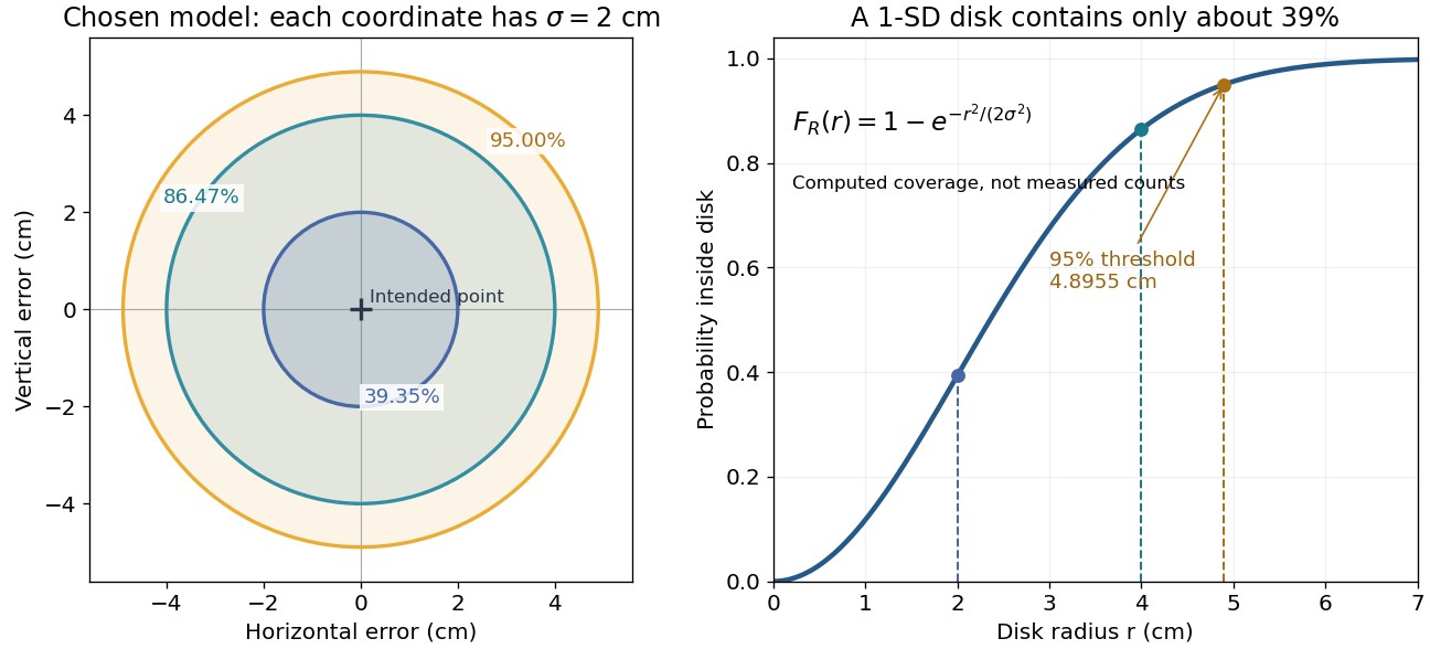
The closed-form quantile function also gives inverse transform sampling: if $U$ has uniform distribution on $(0,1)$, then $\sigma \sqrt{-2\log U}$ has Rayleigh distribution. Using $1-U$ instead gives the same law. Endpoints are excluded so that the logarithm stays finite.

The joint probability density of $X,Y$ isIn polar coordinates, $x=r\cos \theta$, $y=r\sin \theta$, and the absolute Jacobian determinant is $r$. Thus the joint density of radius and angle factors asIntegrating over angle gives the Rayleigh distribution. The same factorization shows that the angle has uniform distribution and is independent of the radius. This is a short change of variables argument: an annulus of width $dr$ has area $2\pi rdr$ to first order.

The assumptions are substantive. Unequal component variances give elliptical rather than circular density contours; a nonzero mean displaces the center. Even zero covariance and equal normal distributions do not suffice without independence. For an original counterexample, let $X\sim N(0,{\sigma }^2)$ and let $S$ be an independent Rademacher random variable. Put $Y=SX$. Then $Y$ has the same normal distribution as $X$, and $\mathrm{Cov}(X,Y)=\mathbb{E}[S{X}^2]=0$. Nevertheless, all points lie on $y=x$ or $y=-x$, and $R=\sqrt{2}|X|$ has densitywhich is positive at zero, unlike the Rayleigh distribution. This pair is not a Gaussian random vector.

Let $a,b,c\in {\mathbb{R}}^n$, with $c\ne 0$. The equation $x=a+(b\cdot x)c$ is the linear system $(I-c{b}^T)x=a$, a rank-one matrix update of the identity matrix. Every solution has $x=a+\lambda c$. Substitution reduces the entire problem toIf $b\cdot c\ne 1$, there is one solution, $x=a+c(b\cdot a)/(1-b\cdot c)$. If $b\cdot c=1$ and $b\cdot a=0$, every $\lambda \in \mathbb{R}$ works and the solution set is the straight line $a+\mathbb{R}c$. If $b\cdot c=1$ and $b\cdot a\ne 0$, there is no solution.

The first reduction follows directly from the original equation in any dimension. In three dimensions it can also be obtained by taking the cross product with $c$, giving $(x-a)\times c=0$. The singular denominator therefore represents two different possibilities, inconsistency or a family of solutions, and must not simply be discarded as an undefined formula.