The released examiner commentary is not a complete worked solution set. It records an accepted ambiguity in question 8(d); question 7(e) also requires care about its unstated drag model.[ref]
https://www.whatdotheyknow.com/request/natural_science_tripos_physics_e/response/2127325/attach/3/FOI%202022%20639%20Sullivan%20materials.pdf?cookie_passthrough=1#page=61. Examiner commentary for this paper, released PDF pages 61–64
By dimensional analysis, power has dimensions , mass density has dimensions , and angular velocity has dimensions ; radians are dimensionless. ThusMatching the three independent dimensions gives , and , henceWith unchanged mass density, angular velocity and the same performance coefficient (a dimensionless quantity), the pump power affinity law givesThe required power therefore increases by . This uses the stipulated dependence on only these three quantities, with comparable pump geometry and performance; dimensional analysis alone does not guarantee that unrelated pumps have the same performance coefficient.
The relativistic kinetic energy is the total energy minus the rest energy:Here is the Lorentz factor and the speed of light. The binomial series, with , givesFor , the leading term is the classical kinetic energy . The ratio of the fourth-order term to that leading term is . ConsequentlyThe condition concerns one term of the binomial series; it is not the condition that the entire relativistic correction be exactly .
Let be signed displacement along the rails, measured from the centre. The diagram in the original paper shows a guide extending across the centre, so the signed coordinate can pass through zero. Hooke's law gives the radial force . In the rotating reference frame, the radial centrifugal force is . The Coriolis force is perpendicular to the rails and is balanced by their reaction; it has no radial component. Therefore Newton's second law givesEquivalently, the radial component of acceleration in polar coordinates in the inertial frame is . The radial spring oscillator on a rotating guide has simple harmonic motion only when , withThe angular frequency is in and the frequency in . The critical angular speed isStrictly this is an upper bound, not an attained maximum for oscillations: at equality , so a displaced object released from rest stays at its displaced position relative to the rails; above it, the central equilibrium is unstable.
Take the thin lens at , with the object on the left and light rays travelling to the right. The positive object distance is and the focal length is . The thin lens equation givesThe transverse magnification and signed image height areThus the real image is beyond the lens, inverted and high. For the ray tracing, a light ray parallel to the optical axis emerges through the far optical focus; a light ray through the optical centre continues straight in the ideal thin lens model. They intersect at , independently reading off both answers from the diagram.
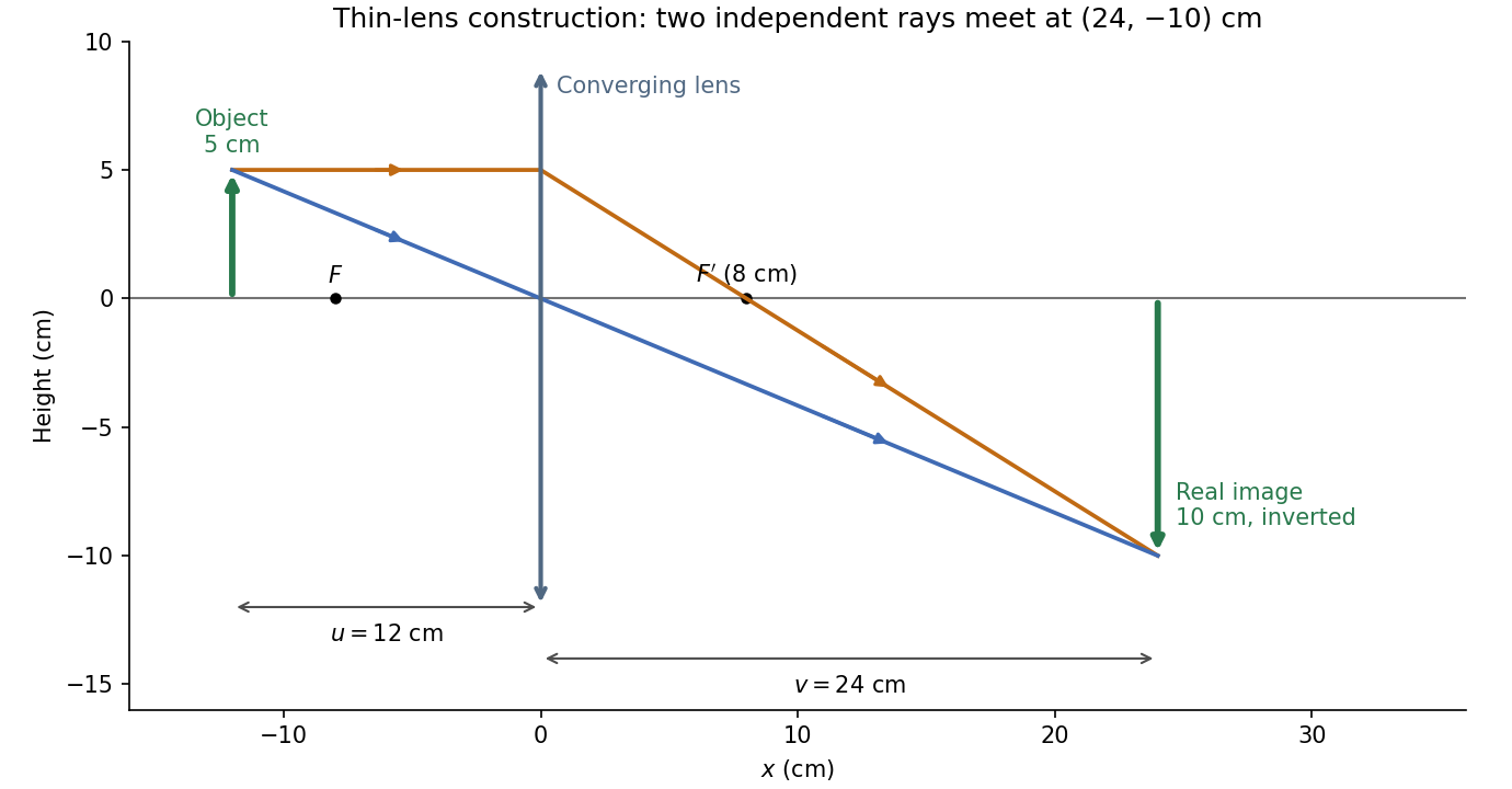

The calculation and diagram use the ideal paraxial approximation implicit in the thin lens equation. The comparatively large object height does not supply enough information to calculate optical aberrations of a real lens.
Write for the side length. In an equilateral triangle, the distance from centre to a vertex is ; it is two thirds of the altitude . By the superposition principle, the electric potential at the centre due to the three fixed Electrons isHere is the elementary charge and the vacuum permittivity. The approaching Electron has electric charge , so its potential energy, measured relative to infinity, is positive:The fixed sources do not move, and radiation is excluded. Hence conservation of mechanical energy givesUsing , for the electron mass, and givesThis speed is small enough to justify classical kinetic energy. There is an idealization in the word “stops”: along the line normal to the triangle through its centre, this threshold energy makes the Electron approach the central equilibrium asymptotically. A smooth, conservative trajectory cannot reach an equilibrium with exactly zero velocity in finite time unless it was already there. The energy threshold, and therefore the requested initial speed, is nevertheless unambiguous.
Choose three mutually perpendicular axes through the same point, and label coordinates . The moments of inertia of any rigid body areSubtracting givesFor a thin planar lamina lying in , the right-hand side vanishes, proving the perpendicular axis theorem:The two in-plane axes and the perpendicular axis must intersect at one point; this need not be the centre of mass. For an extended three-dimensional mass distribution, the equality generally fails. The general moment-of-inertia triangle inequalities arewith equality in the first precisely when all mass lies in the plane perpendicular to its axis, and cyclically for the others. None of these identities requires principal axes.
Let denote the moment of inertia normal to the disc and that about any central diameter. Rotational symmetry makes the two perpendicular diameter values equal. By the perpendicular axis theorem, . The intended angular impulse has magnitude ; delivering that magnitude about a diameter instead gives . ThusThese are principal axes, so angular momentum is parallel to angular velocity in both cases. Equal delivered angular impulse means equal magnitude of the change in angular momentum, not equal rotational kinetic energy; the actual rotational kinetic energy is twice the intended value.
Take along the upper ship's initial velocity, and take from the lower ship to the upper ship at closest approach. The upper and lower ships then have initial velocities and . Their equal masses put each at distance from the centre of mass, soBy momentum conservation, the centre of mass keeps moving with constant velocityIn that frame the ships have opposite velocities of magnitude . Their initial angular momentum about the centre of mass is nonzero even though their trajectories were straight:The tether exerts central internal forces, so conservation of angular momentum givesEach ship follows uniform circular motion of radius around the translating centre of mass, clockwise viewed from . More explicitly, put the initial centre at the origin and defineThe kinetic-energy decomposition about the centre of mass verifies conservation of mechanical energy directly:At closest approach the relative radial velocity is already zero, so connecting the tether requires no dissipative radial impulse. Subsequently its tension is perpendicular to each ship's velocity relative to the centre of mass and does no net work on the pair at fixed .
Each ship needs centripetal acceleration , supplied entirely by the tension. ThusThe result has units of force, .
During quasi-static tether contraction, momentum conservation keeps constant and conservation of angular momentum keeps constant. To leading order in the slow radial motion, the kinetic energy isIts derivative at fixed , not fixed , isTo compute the power supplied by the tension, use the instantaneous unit vector from the lower to the upper ship. Their radial velocities relative to the centre of mass are , and the tension forces are . ConsequentlyThe translational contributions cancel between the two ships and the tangential contributions are zero. The contraction mechanism supplies positive work, increasing the rotational kinetic energy.
The slow-contraction approximation matters: for a prescribed smooth with a taut tether, the exact kinetic energy and tension include radial terms,These still satisfy . Thus the paper's displayed formula is the leading result for slow, smooth contraction, or is exact when the radial kinetic energy is constant; it is not an identity for every possible shrinking schedule.
The mass and surface area of the spherical droplet are and . Constant surface mass accretion rate meansTherefore , and the initial radius givesHere , , and . This surface-fed growth of an accreting sphere law assumes constant droplet mass density.
Choose downward velocity positive, and assume the collected material is initially at rest in the cloud's inertial frame. This assumption is required for the equation in the question. During , momentum conservation for the droplet plus the material it collects givesup to second-order increments. Thus the variable-mass system satisfiesSince , , givingThe notation is appropriate because here depends only on time. The extra term accounts for the momentum needed to accelerate newly collected mass; using would omit it. For incoming material with downward velocity , the more general equation is .
Set . The proposed velocity and its derivative areThe remaining term in the linear ordinary differential equation isso the sum is exactly . Also , establishing both the equation and its initial condition:The integrating factor explains where the expression comes from:The result has units of velocity. Its continuous limit is , despite the apparent in the written expression.
Introduce the dimensionless quantities and . ThenThe Taylor series at givesThus the initial slope is , as for free fall. At late times,The oblique asymptote is , approached from below. Direct differentiation givesThe speed increases monotonically with decreasing slope, from towards . It does not reach a terminal velocity in this drag-free model. Without mass accumulation, and still without drag, a drop released from rest has : its acceleration remains , whereas the growing drop continually shares its momentum with newly acquired material.
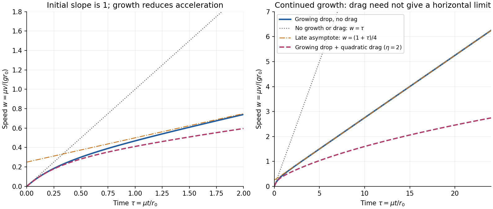
Growing-droplet speed, its early and late limits, and an explicitly assumed quadratic drag example
. Details. 
An upward drag force changes the variable-mass system equation toFor an ordinary drag force increasing with positive speed, the new curve lies below the no-drag curve. It still starts with slope if at rest. The dashed curve illustrates quadratic drag on a sphere with constant radial growth, using with constant drag coefficient and air mass density . The equation for these dimensionless quantities isThe figure uses solely to show the shape; it is not an additional datum of the paper.
There is a limitation to the usual terminal velocity sketch here. The examiner's commentary describes a curve approaching terminal velocity, but the paper maintains unbounded radius growth and specifies no drag law. A horizontal limit is justified if one additionally treats the radius as approximately fixed, or otherwise assumes a drag-to-mass ratio with a fixed limiting balance. With the growing radius and constant- quadratic drag just written, the late balance instead givesThis curve flattens in the sense that its slope tends to zero, but its speed remains unbounded. Thus a lower, more strongly flattening curve is warranted; a finite terminal speed requires an additional assumption. The no-growth approximation gives the familiar finite value for a specified fixed radius.[ref]
https://www.whatdotheyknow.com/request/natural_science_tripos_physics_e/response/2127325/attach/3/FOI%202022%20639%20Sullivan%20materials.pdf?cookie_passthrough=1#page=62. Examiner commentary, B7, released PDF page 62: the stated terminal-velocity expectation
For electric potential difference and electric current varying as sinusoids, choose the phasor conventionThe electrical impedance isIts modulus gives the voltage-to-current amplitude ratio, and its complex argument gives the voltage-minus-current phase difference. For ideal components,These follow from Ohm's law , the capacitor law , and the inductor law . In phasor notation a time derivative becomes multiplication by , turning the linear ordinary differential equations of the electrical circuit into algebraic equations. Electrical impedances add in a series circuit; their reciprocals, the electrical admittances, add in a parallel circuit. This computes both amplitudes and phase differences in the steady response to sinusoids.
The original diagram has a series circuit containing and , in parallel with ; it is not three separate parallel components. The electrical admittance is thereforeFor , voltage and current are in phase when the imaginary part of vanishes. Excluding the zero-frequency solution, division by givesA nonzero lossy parallel coil resonance exists only if . With , and ,For zero electrical resistance, the ideal parallel inductor-capacitor cancellation occurs atThe fractional reduction relative to the zero-resistance coil isAt exactly and , , so finite applied voltage draws zero net current in the ideal model. The quoted frequency is the limiting parallel-resonance value; the phase of an exactly zero current is undefined.
Let be the total parallel capacitance, since capacitors in a parallel circuit have additive capacitances. Put into the lossy parallel coil resonance condition:The additional capacitance is thereforeThis is the added capacitance, rather than the new total, and the conversion from frequency to angular frequency is essential.
For a long solenoid, solenoid inductance obeys , where is the number of turns, the cross-sectional area and the axial winding length. The natural reading of half as many turns occupying half the axial length givesWith unchanged wire material and gauge, halving the wire length also halves its electrical resistance: . With the total capacitance fixed, the new angular frequency satisfiesThusNeglecting the small resistive correction gives the estimate .
There is a documented alternative interpretation: if half the turns are distributed over the original axial length, then while , givingThis corresponds to treating “length of the winding” as wire length while preserving axial geometry. The examiner's report explicitly accepted either inductance scaling, provided the resistance change was included. The first interpretation follows the statement that the axial winding length is halved; the second records the accepted ambiguity rather than silently choosing a different geometry.[ref]
https://www.whatdotheyknow.com/request/natural_science_tripos_physics_e/response/2127325/attach/3/FOI%202022%20639%20Sullivan%20materials.pdf?cookie_passthrough=1#page=63. Examiner commentary, B8(d), released PDF page 63: both inductance scalings accepted, with resistance halved
The Time-independent Schrödinger equation is the energy eigenvalue equation for a particle of mass . The Hamiltonian operator is the sum of the kinetic operator and the prescribed potential energy . Here is the reduced Planck constant. A corresponding stationary state is . The Born rule identifies as probability density for a state with wavefunction normalization ; integrating it over an interval gives a position probability. A plane wave scattering state is not a normalizable wavefunction on the whole line, but its probability currents give the reflection and transmission fractions of an incident wave packet.
There is a notation discrepancy in the sources: the original PDF prints an unbarred in the kinetic term, whereas the local TeX uses . The standard physical equation uses the reduced Planck constant , where is the Planck constant; that convention is used below. Reading the printed literally as the Planck constant would scale all lengths in this model by relative to the standard answers, but would leave the amplitude ratios unchanged.
For , both sides allow oscillatory wavefunctions. A classical particle always crosses the potential step and slows because its kinetic energy falls from to . In quantum mechanics there is generally both reflection and transmission even though the particle is above the step. Define the positive wavenumbersWith no wave incident from the right, writeA finite potential step with constant mass makes both the wavefunction and its first derivative continuous. The two boundary conditions at areSolving gives the reflected and transmitted wavefunctionsFor the specified Electron energies, , so the relative probability amplitudes areThe transmitted probability amplitude exceeding one is compatible with conservation of quantum probability, since the outgoing speed is smaller. In fact the probability current givesThese are the quantum reflection probability and transmission probability, which must be distinguished from the requested relative amplitudes.
Classically, a particle with is completely reflected and never enters the raised region. In quantum mechanics the wavefunction penetrates the classically forbidden side as an evanescent wave. Define the tunnelling decay constantBoundedness at positive infinity excludes , soMatching the wavefunction and its derivative givesThe reflected probability amplitude has unit modulus, hence quantum reflection probability one. The decaying tail carries zero probability current: this semi-infinite potential step has no transmitted beam at infinity, unlike a finite potential barrier. The sketch shows an exact matched example rather than attempting to assign a single real value to a complex wavefunction.
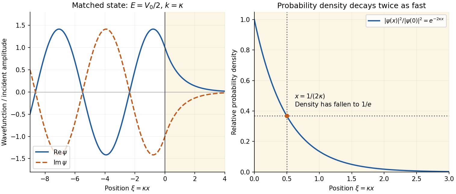
Real and imaginary components of a matched wavefunction at a potential step, with exponential decay of the probability density
. Details. 
Because the probability density decays as , the requested penetration distance isFor a proton, take , and . ThenThe wavefunction amplitude decay length is twice this value. The nonrelativistic equation supplied in the paper is appropriate for this estimate since is small compared with the proton rest energy, approximately . If the original PDF's unbarred is instead read literally as the Planck constant, the displayed differential equation gives . This is a valid calculation for that literal coefficient, but is the physical estimate using the standard Schrödinger equation.
A scanning tunneling microscope brings a tip and surface, both electrical conductors, close enough to leave only a small vacuum gap. An applied electric potential difference makes occupied Electron states on one side able to feed unoccupied states on the other. Although the gap is a classically forbidden potential barrier, quantum tunnelling through its finite width produces an electric current.
For an approximate rectangular potential barrier of gap width , the transmission probability, and thus the electric current at fixed small bias, varies approximately as . This strong distance dependence makes the device sensitive to changes in separation on the scale of a chemical atom. Feedback control moves the tip vertically to keep the electric current constant during a scan; the required height changes form an image of the surface, with contrast also depending on its electronic states. The finite gap permits transmitted probability current, whereas the semi-infinite step in part (b) does not.
For an infinite straight wire in vacuum, Ampère's circuital law around a circle of radius gives . ThereforeHere is the vacuum permeability and the azimuthal direction follows the right-hand rule around the electric current. The magnetic field is measured in .
Choose the electric current counterclockwise as viewed from ; reversing it reverses the magnetic field. Parameterize the circular wire byThe cross product in the Biot-Savart law isConsequently the transverse terms integrate to zero over , while the axial term is constant:ThusThe direction is on both halves of the axis for this electric current orientation, including ; it is not “away from the plane” on both sides. The right-hand rule gives the same direction.
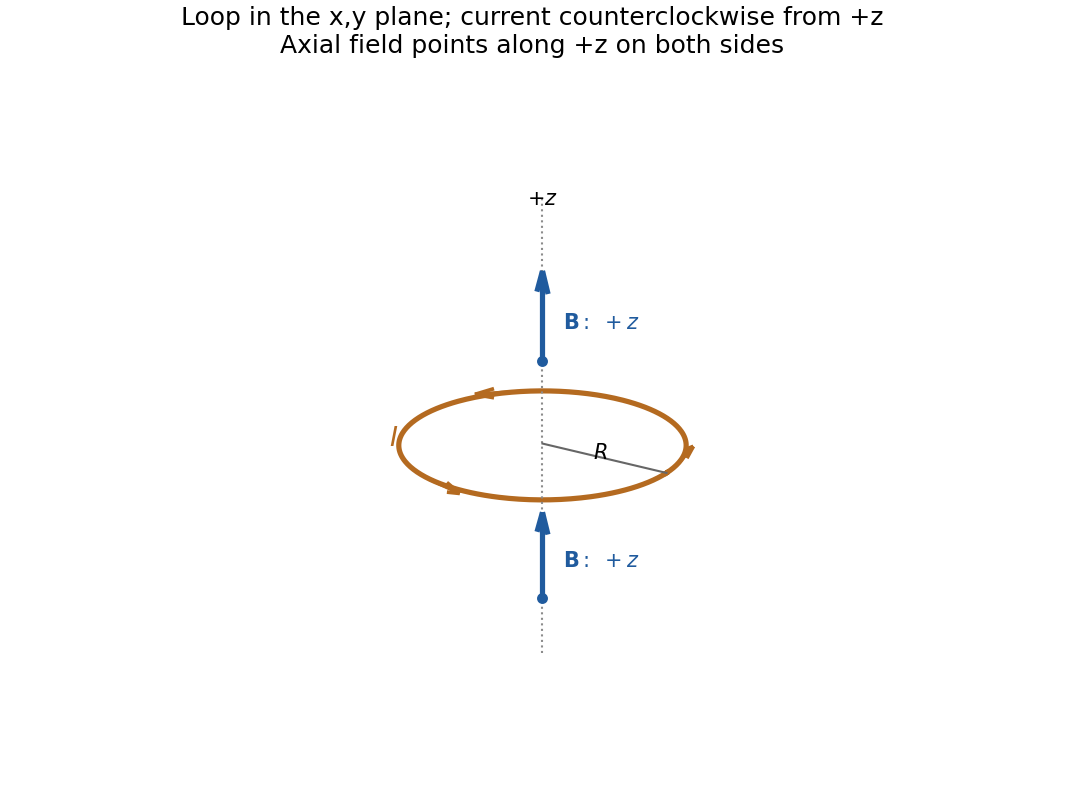
Direction of the axial magnetic field of a circular current loop, with counterclockwise electric current viewed from
. Details. 
Read the original diagram as a clockwise arc carrying electric current from its upper endpoint to its lower endpoint, with tangent semi-infinite leads extending to the right. Their crossing is insulated, so there is no extra junction. Choose out of the page. At the centre the arc produces a negative axial magnetic field, and each straight lead a positive one, by the right-hand rule.
For the arc, every element is at distance , with perpendicular to its displacement to the centre. The Biot-Savart law therefore givesFor each straight lead, write for distance along the tangent measured from its endpoint. Its perpendicular distance from the centre is , soThe integral equals because an antiderivative is . Adding both leads and the arc,Using the full infinite-wire magnetic field for either lead would incorrectly double its contribution.
To calculate magnetic-field cancellation of an arc and tangent leads away from the plane, put . Each point on the arc is distance from , and the axial component of still has magnitude . Thus its axial magnetic field isFor either tangent lead the axial numerator remains , while the cubed distance is . HenceAdding both leads givesFor , a binomial series yieldsThe exact condition for cancellation of the axial component isFor example, keeping would leave a small positive axial magnetic field proportional to . Both contributions weaken with height, but the arc factor is whereas the lead factor is . The arc therefore loses a greater fraction of its axial magnetic field. Increasing its angle compensates for this loss. Physically, the arc is all at the same finite radius, whereas distant elements of the semi-infinite leads undergo a smaller fractional change in distance on moving a little out of the plane.
The cancellation here concerns only; off the plane it does not assert that every component of the magnetic field vanishes. The small-height result also stays within the tangent-lead geometry shown in the original paper.
The released examiner commentary gives performance observations rather than complete worked solutions. Questions 6 and 7 contain several unlettered tasks.[ref]
https://www.whatdotheyknow.com/request/natural_science_tripos_physics_e/response/2127325/attach/3/FOI%202022%20639%20Sullivan%20materials.pdf?cookie_passthrough=1#page=50. Examiner commentary for the 2021 IA Physics paper, released PDF pages 50–52
For a simple pendulum in the small-angle approximation, the oscillation period is , soInterpret the quoted random timing error and length error as standard uncertainties, with independent errors and no additional systematic error. For independent measurements, the standard error of the sample mean of the period is . The length has relative standard uncertainty . By propagation of uncertainty,Requiring a relative standard uncertainty no greater than givesFor , the combined relative standard uncertainty is , or ; gives and just fails. Repeating the timing does not reduce the fixed length measurement uncertainty. The stated “accuracy” is consequently a statistical uncertainty target, not a guarantee for every experimental outcome. This is an example of repeated-timing uncertainty in a pendulum gravity measurement.
The original diagram shows two equal balls, each of mass , attached to the fixed upper pivot and light sliding collar by four equal rods. Each ball describes a horizontal circle of radius . The pivot-to-collar distance is , so the upward collar displacement compresses the spring byThus Hooke's law gives a downward spring force on the collar. Let be the tensions in the upper and lower rods attached to one ball. Vertical force balance on the light collar and then on either ball givesThe radial force on one ball supplies its centripetal acceleration:For , adding the vertical-balance results and eliminating the rod tensions givesFor the given centrifugal governor, andHenceThe factor of two in the collar balance matters: both lower rods support the same light collar. The spring force is not an extra downward force of this full magnitude on each ball; its effect on each ball is transmitted through its own lower rod. The formula is the steady spring-loaded centrifugal governor balance.
Let the cylinder length be , cross-sectional area , and the fluid mass density . At floating equilibrium, Archimedes' principle givesFor a small downward displacement from this equilibrium, the displaced fluid volume increases by . The additional upward buoyant force is , and Newton's second law becomesThis is simple harmonic motion, with angular frequency and oscillation periodThe result for vertical oscillations of a floating cylinder is independent of its cross-sectional area and fluid mass density because those quantities cancel using the known immersion fraction. It neglects drag, surface effects and the extra fluid inertia from the motion; the cylinder must remain partly immersed throughout the small motion.
For a diffraction grating with illuminated lines in order , its ideal spectral resolving power isThe two spectral lines have separation and mean wavelength . In first order, , so the Rayleigh criterion requiresWith line density , the ideal continuous estimate for the illuminated width isRounding the required number of illuminated grating lines upward gives lines, conventionally an illuminated width . Using the longer wavelength rather than the mean also gives the same integer requirement. This is the ideal limit set by the resolving power of a diffraction grating; additional broadening from the illumination or observing apparatus could require a larger width.
The tunnel is taken thin enough that removal of its material does not significantly disturb spherical symmetry. For , the enclosed mass isBy the spherical shell theorem, the inward gravitational acceleration has magnitudeThe released gravitational potential energy is the positive work done by gravity while the mass falls from radius to :By conservation of mechanical energy,Inside the cavity, the spherical shell theorem gives zero gravitational field, so the velocity stays constant. The original figure places B and C at opposite ends of a cavity diameter, a distance apart. ThereforeThe quantity has units , so this is a time. There are no numerical values for or in the paper. The transit time is independent of and the falling mass . The cavity's gravitational potential is constant, not necessarily zero; only its gradient vanishes. The calculation is a hollow-sphere gravitational transit.
Translation and rotation. For particles constituting a rigid body, the total linear momentum isThus the total external force governs the motion of the centre of mass. About that centre of mass, the angular momentum and applied torque arewhere primes denote relative positions and velocities. The derivative of the vector is taken relative to nonrotating axes. The inertia tensor relates angular momentum to angular velocity, . For rotation about a fixed unit direction , the moment of inertia is ; it measures the resistance to changing that rotation and gives rotational kinetic energy . The simpler vector relation applies when the rotation axis is a principal axis, not for every orientation of an arbitrary rigid body. These translational and rotational balances must be applied together; a nonzero torque does not replace the net-force equation.
Gyroscope precession. A rapidly spinning gyroscope has a large angular momentum approximately along its spin axis. The torque component parallel to this vector changes its magnitude, while the perpendicular component turns its direction. If the vector undergoes precession with angular velocity , then over its change is the infinitesimal rotation . HenceThis describes direction-changing precession at constant ; any spin-up contribution must be added separately. For perpendicular torque and angular momentum, the precessional component perpendicular to is . The familiar tendency of a supported gyroscope to turn sideways is this vector balance, not the absence of gravitational force.
Wheel-lift threshold without the flywheel. Let be the centre of mass height, half the wheel separation, and the bend radius. The required inward force is , provided by static friction. Let be the summed outer and inner wheel normal forces. Vertical balance gives . Moment balance about the centre of mass givesThe inner wheels lift when . Thus the vehicle rollover threshold isThe stated mass cancels. This assumes the rigid geometry and sufficient static friction specified in the paper; the threshold is set by loss of contact, not by sliding.
Engine flywheel. The moment of inertia of a uniform disc givesIts spin angular speed, spin angular momentum, and turn angular speed at areThe transverse flywheel axis is perpendicular to the vertical turn axis, soTo specify its direction, use right-handed axes forward, to the car's left, and upward, and consider a left turn. Then . Choose the flywheel angular momentum to the car's right, . The car must applyto obtain the required precession. This gyroscopic roll torque in a turning vehicle opposes the outward roll tendency in a left turn. By the right-hand rule, the flywheel must turn counterclockwise viewed from the car's right side toward its centre, opposite to the rotation of wheels rolling forward. Reversing flywheel spin would aggravate the outward roll. Reversing the turn reverses both roll and gyroscopic torques, so the same flywheel spin remains helpful.
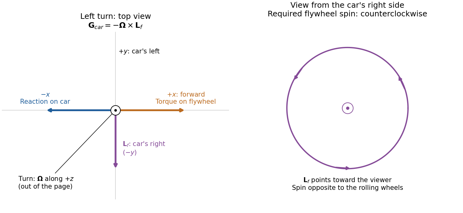
Gyroscope vector directions for a left-turning car and the flywheel spin needed to oppose outward roll
. Details. 
For comparison, the outward inertial roll moment at the stated speed is , and the limiting gravitational restoring moment is . The gyroscopic reaction is about of the former and of the latter, so it is appreciable for this large flywheel. If this ideal model is extended to include the favorable gyroscopic reaction in the wheel-lift condition, it gives , or about rather than . This quantifies a useful but finite increase in the rollover threshold.
Frame definitions and relativistic effects. Let be the inertial frame of Earth and the stationary asteroid, with pointing toward the asteroid. Bob's inertial frame moves at relative to . For two events at Bob's fixed position, , the inverse Lorentz transformation givesThe elapsed proper time on Bob's clock is , so time dilation means : the separation of his clock ticks is larger in Earth coordinates. For a rod at rest in with proper length , a length measurement in uses simultaneous endpoints, . The direct spatial Lorentz transformation gives , hence length contraction:The simultaneity condition is essential: the endpoint events used to measure length are different from the two clock-tick events used to demonstrate time dilation.
Bob's speed. Food consumption measures Bob's own proper time, . The Earth-frame distance is and the Earth travel time is . ConsequentlyPutting , , soThe Earth travel time is months. Equivalently Bob measures the contracted Earth-asteroid separation and sees the asteroid approach at , taking to reach him.
Events A and B. Set both coordinate origins at Event A. Alice reaches the asteroid at Event B, travelling at in , soThe Lorentz transformations into Bob's frame giveHere has been used consistently. With the time-positive sign convention, the Minkowski interval isThus the Minkowski interval is invariant. It is timelike, as expected for two events on Alice's subluminal worldline. Using the opposite metric sign convention would change both signs together, without changing invariance.
Relative velocity and spacetime diagram. Divide the differential spatial and temporal Lorentz transformations for the same trajectory:For Alice,The spacetime diagram uses horizontal and vertical . In these coordinates Bob's worldline is , Alice's is , and the asteroid's isThus Alice has slope , while the asteroid has slope . Their intersection is exactly B, . The asteroid later reaches Bob at . These intercepts and gradients show the relativistic velocity addition geometrically.
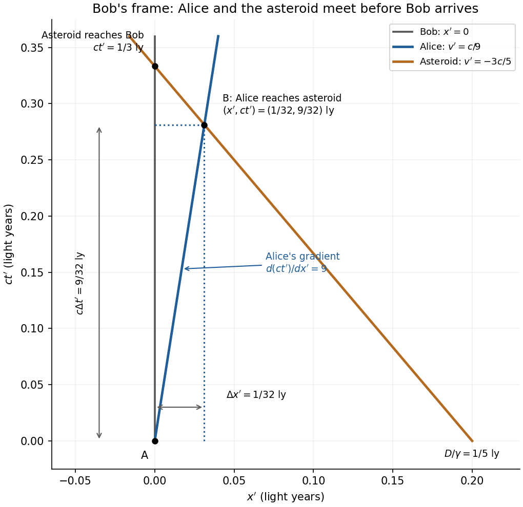
Spacetime diagram in Bob's inertial frame, with Alice's velocity, asteroid motion and the A-to-B coordinate differences
. Details. 
The force law separates into two identical harmonic oscillator equations:For positive , the general real solution isSince by Euler's formula, these are exactly the stated real parts of complex exponentials. The amplitudes and phases are fixed by the four initial position and velocity components. This is two-dimensional isotropic harmonic oscillator flow: the same angular frequency acts in every direction.
Put . If both coordinate amplitudes are nonzero, eliminate the common phase to obtainFor , this is an ellipse centred at the origin. The following special cases exhaust the possible nontrivial shapes:
- or gives straight-line simple harmonic motion, including an axis-aligned line if one coordinate amplitude vanishes.
- gives an axis-aligned ellipse; if additionally , it is a circle traversed in one of the two orientations.
- Other phase differences give tilted ellipses.
The degenerate zero-amplitude solution is the stationary origin. There are no general multi-loop patterns here because the two angular frequencies are equal. Another useful description is , the image of a circle under a linear map.
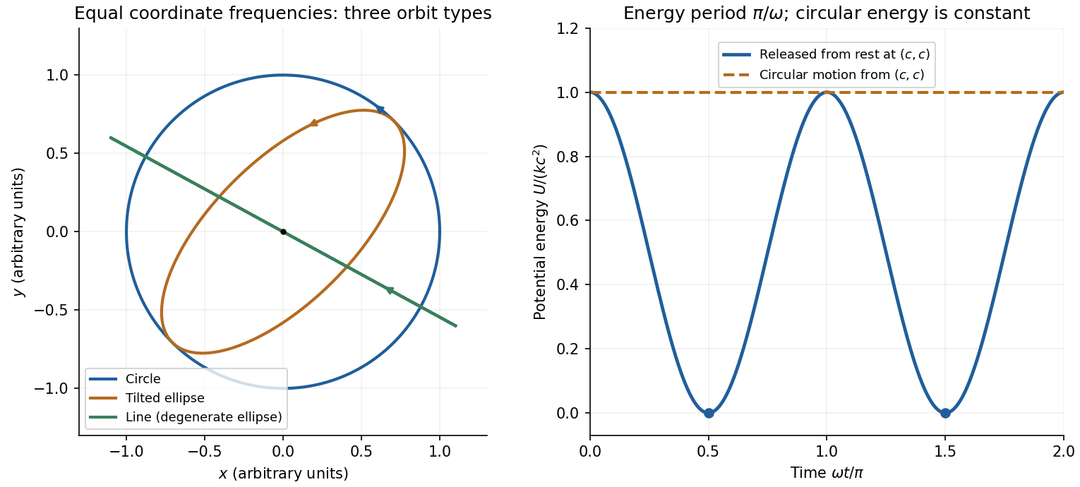
Undamped planar harmonic oscillator trajectories and potential energy for the two specified initial conditions
. Details. 
The force is conservative, with and potential energy zero at the origin:Released from rest at , the trajectory has , givingThe right panel of the figure shows this nonnegative oscillation: it starts at a maximum , reaches zero at , and repeats after . Its frequency is twice the coordinate frequency. Conservation of mechanical energy gives , so the missing potential energy is kinetic energy, not an energy loss.
The starting radius is . In uniform circular motion, the required centripetal acceleration has magnitude . The initial velocity must be tangent to the starting radius, with the orientation chosen anticlockwise:The resulting trajectory isIt has constant , soThis is the horizontal line in the right panel of the figure. The kinetic energy also equals , giving total mechanical energy , twice that for release from rest at the same point.
Write and , where is the undamped angular frequency. The linear drag gives the vector damped harmonic oscillator equationFor the original circular initial conditions, and , the exact underdamped solution isUsing , and givesThis exact potential energy is useful because it satisfies the prescribed initial conditions, including . In the stated weak-damping limit , and the square bracket differs from one by a small oscillatory term. The leading approximation is thereforeThe radius is approximately , so the trajectory is approximately a shrinking logarithmic spiral. The exactly exponential result would require slightly adjusted initial velocity; with the specified undamped circular velocity, the small modulation above is real. This is the initially circular damped planar oscillator.
The parameters giveThe coordinate expressions for the initially circular damped planar oscillator areThe damped oscillation period gives almost four anticlockwise turns in four seconds. The radius envelope falls by . Substitution into the exact coordinates givesThe left panel annotates the initial tangent, time marks and endpoint. Because is an unspecified starting coordinate, the axes are normalized by rather than assigned numerical lengths.
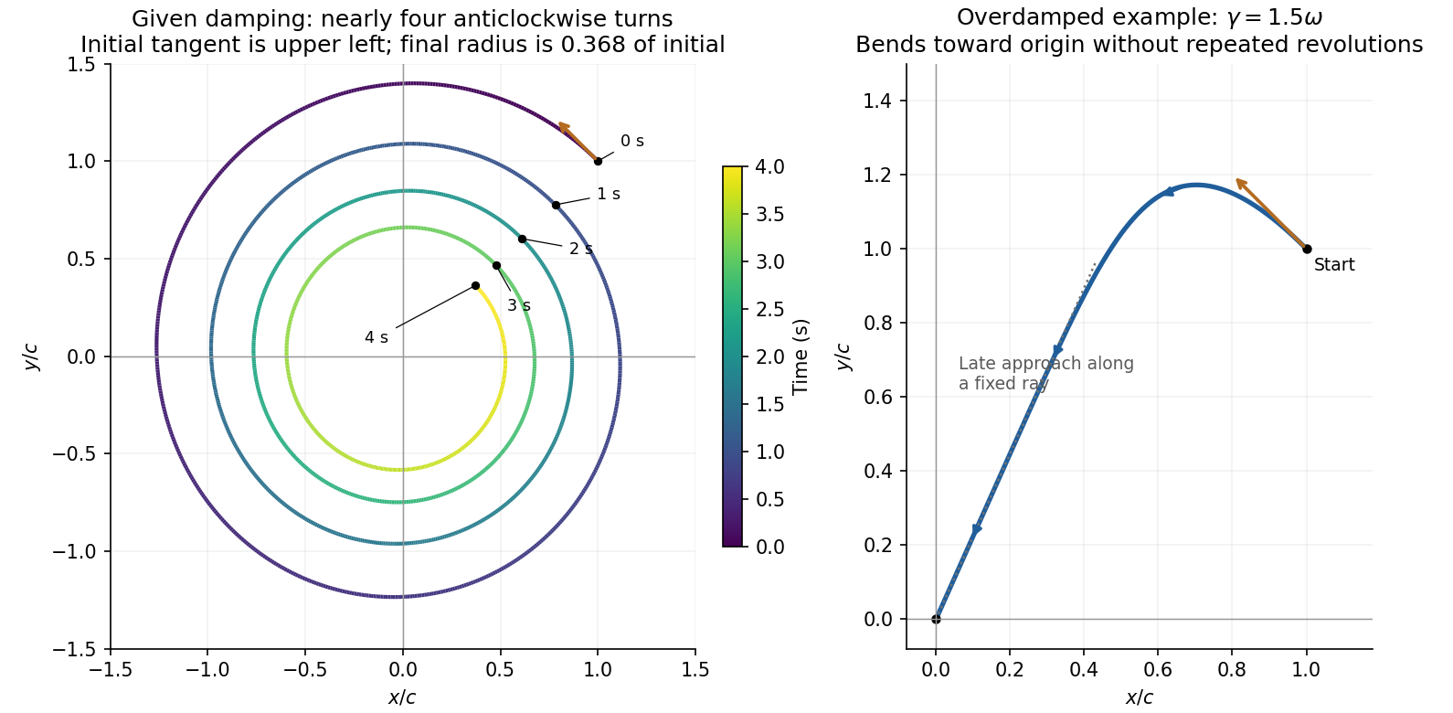
Exact underdamped trajectory over four seconds and a representative overdamped trajectory for the same initial circular velocity
. Details. 
For overdamping, . Put . Both characteristic roots are negative real numbers. Replacing trigonometric functions by hyperbolic functions gives the exact trajectoryIt starts from with tangent , bends anticlockwise toward the origin, and approaches it without repeated revolutions. The right panel gives a representative choice ; the paper does not specify one particular value of in this regime.
One can make the qualitative shape precise. In radial and tangential directions relative to the initial radius, the angle turned from the starting direction obeysFor , both coordinates stay positive, and the approach is along the fixed ray with . The initial velocity is tangential, so an immediately straight radial return would be incorrect. The absence of oscillatory characteristic roots prevents repeated revolutions. This is a non-spiralling overdamped central oscillator trajectory.
Use the original diagram's positive distances: from the object to the vertex, from the vertex to the image, and from the vertex toward the centre of curvature on the outgoing side. Let a paraxial light ray strike at height . Its incoming inclination is above the optical axis, its outgoing inclination is below it, and the inward surface normal is inclined by below it. Thus the incidence and refraction angles relative to that normal are respectively and .
The local tangent-plane form of Snell's law, using the small-angle approximation, givesSubstitute the three height-to-distance ratios and cancel :This refraction at a spherical surface result keeps only first-order ray angles. The surface sag shifts the height's axial reference only at higher order. Distances for other object, image or curvature orientations must be signed consistently; the displayed positive-distance form follows the particular orientation in the paper.
Keep the paper's as magnitudes for the two convex faces. With the standard signed-curvature convention measured to the right, the first surface has signed radius and the second . This explains why the requested formula contains a sum of the two reciprocal magnitudes.
Let the axial lens thickness be , and let be the distance from the first vertex to the intermediate focus that its refracted rays would reach without the second surface. The first refraction at a spherical surface givesAt the second face those rays are still converging toward that intermediate focus, so its object distance is negative, , with . Applying the signed spherical-surface equation again givesIn the thin lens limit, . Adding cancels the intermediate-focus terms:The focal length is the image distance for parallel incident light rays, , hence the lensmaker's equation isThe same surrounding refractive index is assumed on both sides. For this biconvex thin lens has positive focal length. With signed radii , , the equivalent familiar expression is .
Use positive object distance and focal length . The thin lens equation givesThe transverse magnification is , so the signed height isThe real image lies beyond the lens, is inverted, and has positive height magnitude .
Articles were limited to the first 100 out of 230 total.
Articles by others on the same topic
There are currently no matching articles.