
Suppose and , and is an analytic function on a disk of radius strictly larger than . The Taylor series at zero of has radius of convergence . Its coefficients are the sum of and the more rapidly decreasing coefficients of . At , the logarithmic part is an alternating harmonic series and converges conditionally; at it diverges. The power series for converges absolutely at both endpoints and therefore cannot change either conclusion. The real convergence interval is .
For , take and , with its branch normalized by . The quotient has nonzero removable value at . Its next zeros are at , so a holomorphic logarithm exists on a larger disk. This shows why the Taylor series converges at even though its singular positive endpoint is excluded.
Radius of a Maclaurin series from successive derivatives Created 2026-10-18 Updated 2026-10-25
Write the Maclaurin series coefficients as . When the successive ratios exist eventually and have a limit, the ratio test gives the displayed radius of convergence, including zero and infinity. The unconditional formula is , from the Cauchy-Hadamard theorem. Endpoints must be checked separately.
The existence and convergence of this power series do not by themselves imply that it equals : equality requires analyticity or control of the Taylor remainder. The smooth function for , , has all derivatives zero at zero, so its Maclaurin series is identically zero despite the nonzero values away from zero.
Complex visibility 2026-10-18
A complex visibility is a calibrated complex correlation of the signals received at a particular interferometric baseline. In a narrow field, with scalar radiation, the far-field approximation for an outgoing source, a narrow frequency channel, negligible noncoplanar phase curvature and a steady sky of mutually incoherent emitters,Here are small dimensionless sky-direction offsets, is brightness in the chosen channel, and is the primary beam. This is the Fourier transform of beam-weighted brightness. The two-dimensional formula requires those approximations: a wide field generally needs the third baseline coordinate and curved sky geometry.
For an explicit one-dimensional derivation, set the primary beam to one over the small field, and place independent emitters at angular offsets . Choose a wave phase convention in which, after removing the phase centre's delay, their received complex amplitudes areHere is the Kronecker delta and angle brackets denote an expected value estimated by time averaging a steady signal. The last equality states mutual incoherence: different emitters have zero averaged cross term, although each emitter's two received copies remain correlated. Multiplying and averaging givesFor continuous brightness this becomes . Real brightness implies the Hermitian symmetry ; it does not require brightness to be even. In particular, an asymmetric real source usually has a nonzero imaginary complex visibility. At zero baseline, is the total beam-weighted source strength. Ordinary separated-element correlations need not measure that zero-baseline value.
Radio interferometer calibration 2026-10-18
Radio interferometer calibration estimates instrumental and propagation effects that alter a complex visibility. A simple narrow-field model iswhere are complex receiver gains and represents additive noise. A point-like astronomical source of known position and stable strength constrains these gains: its expected complex visibility has a known wave phase and amplitude. A resolved or variable reference source requires a better source model. Errors in the reference model can be transferred into the inferred sky.
In a proposed extension, Martin Ryle described simultaneous observation of a nearby reference point source to correct atmospheric wave phase errors, using an additional dish at each element. He presented this as a possible extension, rather than the standard One-Mile Telescope arrangement.[ref]
Radio Telescopes of Large Resolving Power by Martin Ryle. Ryle (1974), p. 202: proposed reference-source correction
Interferometric baseline 2026-10-18
An interferometric baseline is the displacement between two antennas. For a unit line of sight toward the phase centre, its projection onto the plane of the sky isHere is the speed of light. The signed delay depends on which receiver is delayed; the geometric path difference's magnitude does not. If is a unit tangent in the direction being imaged, the dimensionless coordinate is a spatial frequency, measured in cycles per radian of small sky offset. A single pair gives fringes of angular period along that tangent. This period specifies one measured oscillation; it does not specify a whole image's angular resolution or eliminate ambiguous source arrangements.
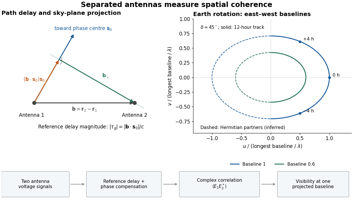
Geometric delay, projected baseline, and a schematic Earth-rotation track; original geometry, not telescope data
. Details. 
The left panel separates the component producing the reference delay from the component measuring angular structure. The right panel shows a possible Earth-rotation aperture synthesis track, with its opposite complex conjugate track. Those opposite samples provide the symmetry required by a real brightness distribution; they are not independent extra observations.
Phase centre Created 2026-10-18 Updated 2026-10-20
The phase centre is the reference sky direction for removing geometric delay and its associated wave phase. An unresolved source exactly there ideally has constant complex visibility after calibration; a displaced source has a baseline-dependent wave phase.
On a shell with homogeneous Dirichlet boundary conditions, put and . The radial heat equation in three dimensions becomes , with zero values at both endpoints. Expanding in a Fourier sine series gives the displayed solution, with . Each radial mode decays at the square of its wave number. The positive inner radius makes division by harmless throughout the shell.
For a classical monatomic homogeneous fluid with pairwise central pair potential , the mean interaction energy is one half the sum over neighbours of a tagged particle. Using the radial distribution function gives the displayed formula; the factor one half prevents counting each pair twice. The kinetic term follows from the equipartition theorem. Its use requires the relevant integral to exist and a thermodynamic state specified by number density and temperature. Quantum kinetic contributions, many-body forces and internal molecular modes require modifications.
Virial pressure from pair correlations Created 2026-10-18 Updated 2026-11-05
For a differentiable central pair potential in a classical homogeneous three-dimensional fluid, the mechanical virial theorem gives the displayed pressure. The radial distribution function accounts for the probability of each pair separation. In the dilute limit, , and integration by parts yields . Thus the second virial coefficient controls . A few virial terms are a low-density approximation, not generally a converged description of a dense liquid. A discontinuous hard core needs its contact form or a limiting argument.
Constituent quark mass Created 2026-10-18 Updated 2026-11-05
A constituent quark mass is an effective mass parameter in a low-energy constituent-quark model. It accounts approximately for strong-interaction dressing and some spin-independent bound-state dynamics; it is not identical to a renormalized quark mass in the Standard Model Lagrangian.
Position uncertainty Created 2026-10-18 Updated 2026-11-05
The position uncertainty of a quantum state is the standard deviation of its measured position, provided the second moment is finite. It is computed from the position operator with the Born rule. An oscillator coherent state has independently of its mean position; translating the state changes the mean without changing this variance.
If a single approximately stationary emitting region changes coherently through a causal disturbance, a disturbance travelling no faster than the speed of light takes at least to coordinate a scale . Light-travel differences also smear simultaneous emission from different depths. Under those assumptions, observed intrinsic variability on a time scale suggests .
For a chosen example , multiplication by gives . This is an order-of-magnitude causality bound on a coordinated emitting scale. It is not a measured stellar radius, and even the relation between and a diameter depends on geometry. A pulsar beam crossing is a geometric clock, and pulsar dispersion delay, scattering and instrumental response can broaden its observed pulse. The recurrence period, observed pulse width and intrinsic variability time must therefore be distinguished before applying the bound. Relativistically moving emitters require further arrival-time corrections.
Pulsar period folding and alias checks 2026-10-18
Phase folding of a light curve collects samples at equal trial phase. Consider a noiseless illustrative pulsar with one pulse every and arrival times , after pulsar dedispersion. At , all arrivals fold to one phase. But also puts all arrivals at one phase: folding discarded the fact that alternate proposed cycles contain no pulse. At , the arrivals instead occupy two phases, and . Thus a sharp folded profile alone need not identify the fundamental period.
Check the original time sequence, adjacent arrival intervals and pulse occupancy as well as the folded profile. With arrivals and a slightly wrong trial period, the unwrapped drift isFor and , this is about cycle. Splitting the observation into early and late pieces reveals the drift that one full folded average can blur. Separately, regular discrete sampling can create aliasing: observing at a spacing comparable with the pulse width can miss narrow pulses even when the recurrence period is much longer. Neither this toy exercise nor one sharp profile replaces time-standard calibration and propagation corrections.
Pulsar dispersion delay Created 2026-10-18 Updated 2026-10-20
A radio wave traversing a dilute cold plasma has a group velocity that depends on its frequency. In the ideal unmagnetized limit, the dispersion relation is , where is the angular plasma frequency. For , differentiate to obtain , then expand to first order. The excess travel time over a vacuum path isHere is ordinary frequency, is the magnitude of the elementary charge, is the electron mass, is the vacuum permittivity, is electron number density, and is the speed of light. This approximation neglects magnetic corrections, collisions and multipath scattering; its positive sign means lower frequencies arrive later.
Discovery of the first pulsar 2026-10-18
Jocelyn Bell Burnell helped build Antony Hewish's radio telescope for finding compact sources through interplanetary scintillation in the solar wind. Operating it and inspecting its chart recorder output in 1967, she recognized an unusual recurring trace, checked earlier charts, and obtained fast recordings resolving pulses in late November. Her observation, recognition and persistent analysis were indispensable.[ref]
Little Green Men, White Dwarfs or Pulsars? by Jocelyn Bell Burnell. Little Green Men, White Dwarfs or Pulsars?, construction through November recordings
The 1968 paper by Antony Hewish, Jocelyn Bell Burnell (bylined S. J. Bell), J. D. H. Pilkington, P. F. Scott and R. A. Collins reported spacing and proposed compact-star oscillations. Its radio telescope had 2,048 full-wave dipole antennas in sixteen rows. Four receivers selected declinations; two array halves formed an east-west interferometer. The receivers passed . Observations used receiver time constant and Rapidigraph chart recorder with time constant; radio second pips calibrated timing.[ref]
Observation of a Rapidly Pulsating Radio Source by Antony Hewish and others. Observation of a Rapidly Pulsating Radio Source, Nature 217, p. 709, opening and Position and Flux Density
Antony Hewish checked sidereal time recurrence. Jocelyn Bell Burnell recalls that P. F. Scott and R. A. Collins reproduced the pulses with another telescope and receivers, while J. D. H. Pilkington measured pulsar dispersion delay: independent checks of instrument independence and intervening plasma.[ref]
Little Green Men, White Dwarfs or Pulsars? by Jocelyn Bell Burnell. Little Green Men, White Dwarfs or Pulsars?, follow-up controls
A useful numerical comparison uses the approximate sidereal time day of . Relative to a schedule, the same sky direction transits about earlier each day, or after ten days. This compares successive passages through the receiving beam; it is a different clock from the roughly pulse spacing within one passage. Sky recurrence alone cannot rule out every transmitter or reflection, and pulsar dispersion delay alone does not uniquely establish an emission mechanism. Their strength lies in independent constraints agreeing.
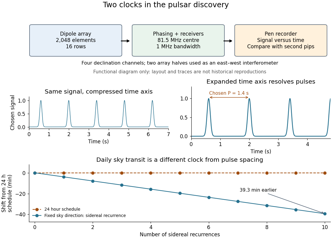

The discovery lesson is that an unexpected signal must survive changes of readout, instrument and observing date. Increasing chart recorder speed exposed structure hidden in a compressed trace; it did not make the source begin pulsing. The pulsar interpretation now separates the rotating clock, beam geometry, pulsar magnetosphere emission and pulsar dispersion delay. The initial observation established periodic arrival, not a direct measurement of the neutron star's surface motion or radius.
Binary pulsar Created 2026-10-18 Updated 2026-11-05
A binary pulsar is a pulsar in a binary star: the companion's gravity changes the emitting neutron star's motion and hence its pulse arrival times. The companion need not itself be a detectable pulsar. Pulsar timing turns that motion into a measurable orbit, making the system useful for stellar mass determination and tests of general relativity.
Pulsar timing Created 2026-10-18 Updated 2026-10-20
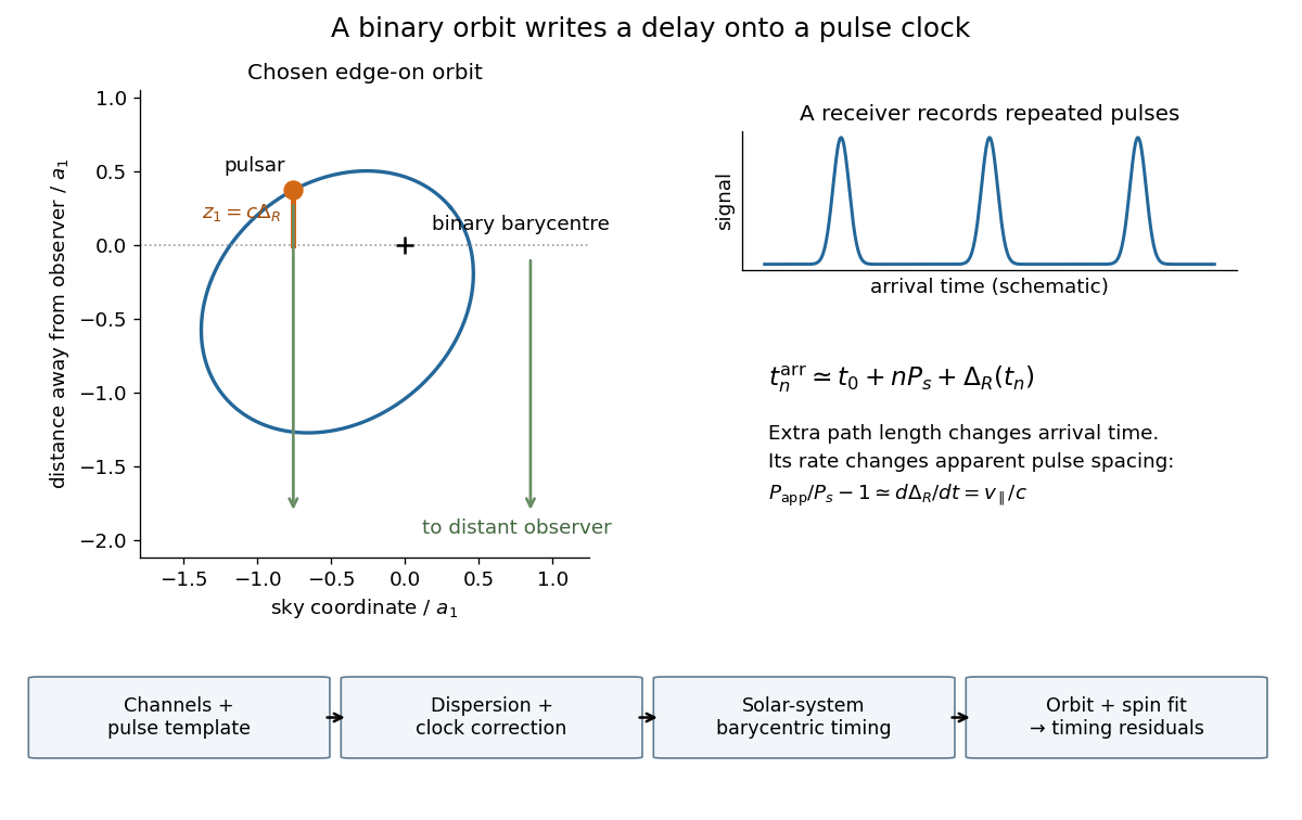
The mature experiment uses channel-template comparison, pulsar dedispersion, GPS clock-offset transfer, Solar system barycenter corrections and connected pulse counts.[ref]
For a geometric illustration, let a perfectly uniform source emit pulse at , with spin period , and let increase away from the observer. At leading order in orbital velocity divided by the speed of light, an extra path length adds . Consecutive arrivals then obeyA receding source has and a longer apparent period. This derivation isolates the geometric Doppler effect; a precision relativistic clock model also needs gravitational redshift and time dilation.

Arginine 2026-10-18
A proteinogenic amino acid represented by R or Arg in protein primary structure. Its amino acid side chain carries predominantly positive electric charge near neutral pH.[ref]
26.1 Structures of Amino Acids. Organic Chemistry by John McMurry; Table 26.1, lysine and arginine rows; side-chain protonation at pH 7.3
Trypsin preferentially cleaves after its amino acid residues.
Lysine 2026-10-18
A proteinogenic amino acid represented by K or Lys in protein primary structure. Its amino acid side chain carries predominantly positive electric charge near neutral pH.[ref]
26.1 Structures of Amino Acids. Organic Chemistry by John McMurry; Table 26.1, lysine and arginine rows; side-chain protonation at pH 7.3
Trypsin preferentially cleaves after its amino acid residues.
For the prolate spheroid with , intersect the concentric sphere . When , subtraction gives two circles in the perpendicular planesTheir centers lie on the long principal axis and the line through the centers is normal to both planes. At the circles merge into the equator; at they shrink to the two polar vertices. There is no intersection for or .
There are unlisted articles, also show them or only show them.