
Half-harmonic oscillator Created 2026-10-18 Updated 2026-11-05
A half-harmonic oscillator has on and an infinite wall at . Its wavefunction vanishes at the wall. Only the odd full-oscillator energy eigenstates satisfy this condition; restricting them to the positive half-line and multiplying by restores normalization. Thus for . With , its normalized ground state isIt has no interior node on its allowed half-line, and energy .
Work by Pyotr Leonidovich Kapitza Created 2026-10-18 Updated 2026-10-25
Ballistic orbit insertion with constant gravity Created 2026-10-18 Updated 2026-10-20
In the flat-surface, constant-gravitational acceleration model, a coasting projectile conserves horizontal velocity. If it arrives at the top of its trajectory with horizontal speed , its earlier velocity at angle above the horizontal has vertical component . Its remaining height gain is therefore . The displayed burnout height follows. This is a local projectile motion approximation, not an exact Kepler orbit. Computing assumes constant gravitational magnitude also at the orbit; computing instead assumes an inverse-square law with surface value . Those assumptions must be distinguished.
Amplitude spectral density Created 2026-10-18 Updated 2026-10-25
An amplitude spectral density is the square root of a power spectral density. For an electric potential difference expressed in volts and frequency in hertz, its units are .
Complex potential of a two-dimensional potential flow Created 2026-10-18 Updated 2026-11-05
For an incompressible irrotational two-dimensional potential flow, an analytic complex potential of a two-dimensional potential flow combines the velocity potential and streamfunction . The Cauchy-Riemann equations give and , hence . Curves of constant are streamlines. An analytic coordinate change transforms the complex velocity by wherever .
Potassium-40 2026-10-18
Potassium-40 is a long-lived radioactive isotope with 19 protons and 21 neutrons. It can decay to calcium-40 through beta-minus decay, or to argon-40 through electron capture and a rare beta-plus decay. The argon-producing branch supports potassium-argon dating.
Position vector 2026-10-18
A position vector is the vector from a chosen origin to a point. Its time derivative is the velocity; differences of position vectors give displacement.
Agarose 2026-10-18
A polysaccharide that forms a porous gel on cooling from solution. In agarose gel electrophoresis, the agarose network provides a size-dependent obstacle to DNA migration in an electric field.
Agar 2026-10-18
Repeat the random evaluation test for a polynomial identity with fresh independent random variables, keeping the same fixed polynomial. Reject as soon as any polynomial evaluation is nonzero; accept only if all values vanish. An identity is always accepted, preserving one-sided error. If a nonzero polynomial has single-trial false acceptance probability , independence gives . The Schwartz-Zippel lemma bounds this by when .
For over the finite field , two uniform independent choices have equally likely ordered outcomes, each with probability . Both polynomial evaluations are zero only at . Hence false acceptance falls from in one trial to in two trials, and correct rejection rises from to .
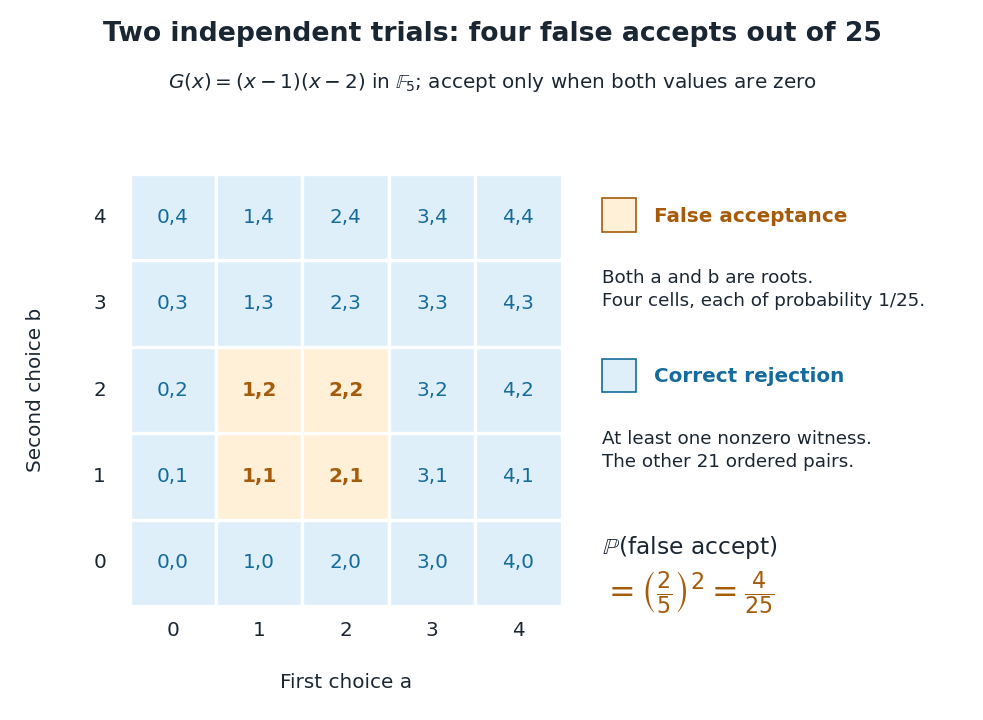
Four of the twenty-five independent pairs falsely accept the nonidentity
. The orange cells have both coordinates among the polynomial roots one and two of in the finite field . Every blue cell supplies at least one nonzero witness. The full grid enumerates exact outcomes under independence and a uniform distribution on a finite set; it is not a simulation. Details.
If the second choice reuses the first, the pair is and only five diagonal outcomes are possible. Two still falsely accept, so the error remains . Choosing fresh independent points is precisely what makes the full -cell grid and the product of probabilities valid. For a target error , this example needsThe ceiling function makes the trial count an integer. Four trials give , while six give ; five still give , so six is the first count below one percent. This is an exact error guarantee for each run on , rather than an observed success rate.
Let be a nonzero multivariate polynomial over a field , with total degree at most . Choose a nonempty finite set . For independent random variables , each with a uniform distribution on a finite set on , the Schwartz-Zippel lemma givesNonzeroness is essential; the zero polynomial always evaluates to zero. The total degree sums exponents within each monomial, rather than taking their maximum: has total degree five. The field need not be finite, but must be finite. The estimate reduces error only when .[ref]
CMPT 710 - Complexity Theory: Lecture 18. CMPT 710 and CMPT 407 - Computational Complexity - Fall 2007; CMPT 710 - Complexity Theory: Lecture 18, §3.1, pp. 3–4: Lemma 4 and its inductive proof
The proof begins with the root bound for a polynomial. For several variables, write , with . The total degree of is at most . By induction, vanishes with probability at most . Otherwise the remaining univariate polynomial has at most polynomial roots. Adding the two contributions gives .[ref]
CMPT 710 - Complexity Theory: Lecture 18. CMPT 710 and CMPT 407 - Computational Complexity - Fall 2007; CMPT 710 - Complexity Theory: Lecture 18, §3.1, pp. 3–4: split by the leading coefficient in the last variable
The algorithm samples a point, performs exact polynomial evaluation, rejects the identity if the value is nonzero, and otherwise accepts. The lemma bounds false acceptance for every fixed nonzero input. For the polynomial identity testing over a finite field example, has and , so its exact error attains the bound. Numerical near-zero values from floating-point arithmetic do not satisfy this exact algebraic contract. A polynomial-time algorithm claim additionally needs efficient sampling and evaluation, including the bit cost of representing and operating on field elements. Counting field operations alone does not establish that cost.
Work in the finite field , using modular arithmetic modulo five. Consider the two original polynomial examplesThe distributive property gives , so all coefficients of cancel: is identically zero. In contrast, in this finite field, with nonzero leading coefficient. Its roots of a polynomial are exactly one and two: a product in a field is zero only if a factor is zero.
The complete polynomial evaluations, displayed as representatives modulo five, areIn particular, is a nonzero witness, which disproves identity without examining other points. At one or two, a zero value fails to reveal that is nonzero. A random variable with a uniform distribution on a finite set hits those two polynomial roots with probability .
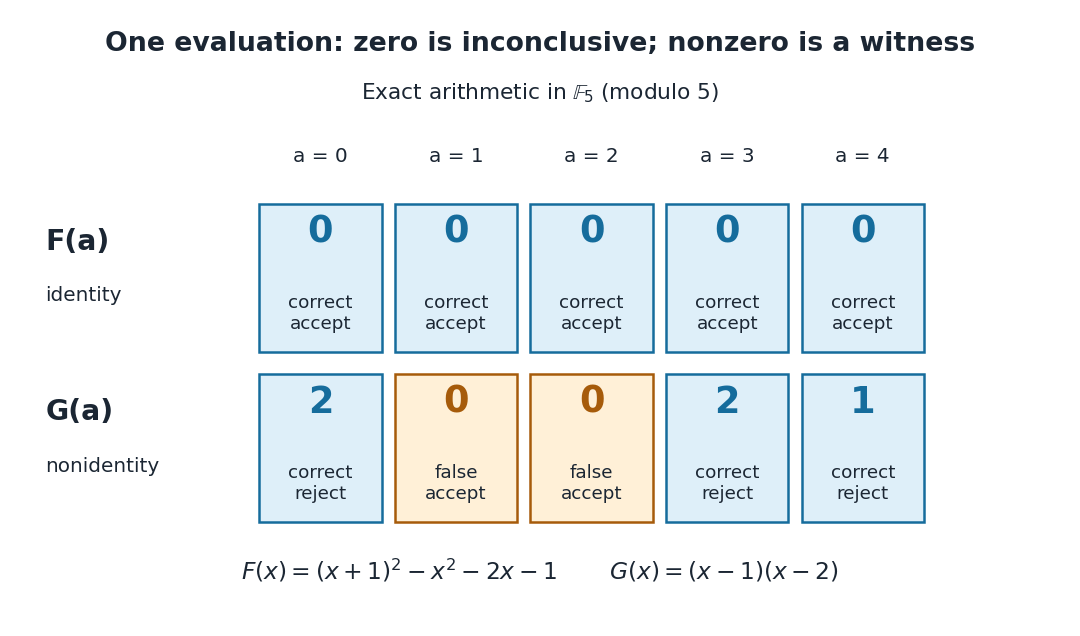

A crucial limit appears with . Its coefficients make it a nonzero polynomial of polynomial degree five in , yet direct polynomial evaluation gives zero at all five field elements: the values before reduction are , all divisible by five. Thus induces the same polynomial function as the zero polynomial. Any number of trials restricted to will falsely accept this identity. This is compatible with the Schwartz-Zippel lemma: the ratio of polynomial degree to sampling-set size is , which gives no useful guarantee.
When a polynomial's representation permits polynomial evaluation over a larger field extension, a larger sampling set can restore the useful degree ratio. Access only to the induced polynomial function on the original finite field cannot distinguish from zero.[ref]
Lecture 9: Polynomial Identity Testing by the Schwartz-Zippel Lemma. CPSC 536N: Randomized Algorithms; Lecture 9: Polynomial Identity Testing by the Schwartz-Zippel Lemma, §1.4: formal nonzero polynomials can vanish everywhere on a finite field; extension-field evaluations need a suitable representation
Univariate polynomial 2026-10-18
A polynomial in one indeterminate; its coefficients lie in a specified ring. For example, is univariate, whereas involves two indeterminates.
Cubic polynomial 2026-10-18
A cubic polynomial in one variable has polynomial degree three. Over a splitting field, its factorization of polynomials contains three polynomial factors of polynomial degree one when multiplicity of a root is counted.
Vieta's formulas Created 2026-10-18 Updated 2026-10-20
Vieta's formulas connect two descriptions of a polynomial: its coefficients and its roots of a polynomial. They let us read the sum and product of the roots of a polynomial without finding the individual roots of a polynomial, and turn a proposed factorization of polynomials into checkable coefficient identities. The key is that coefficients encode elementary symmetric polynomials, which are unchanged by a permutation of the roots of a polynomial.
For a polynomial of polynomial degree , with nonzero leading coefficient , write its factorization of polynomials in a splitting field asList every root of a polynomial according to its multiplicity of a root. ThenIn particular, and . With coefficients in the real numbers or complex numbers, the fundamental theorem of algebra ensures that a list of roots of a polynomial in the complex numbers exists when multiplicity of a root is counted.[ref]
For a monic polynomial, this is the familiar conventionwhere is the th elementary symmetric polynomial in the roots of a polynomial; in particular, . The ratio by in the general statement matters: multiplying every coefficient by the same nonzero scalar preserves both the roots of a polynomial and these ratios.
A short derivation explains every alternating sign. In the product , a term of polynomial degree arises by choosing from distinct factor positions and from the others. Summing the resulting products gives . Values at different positions may coincide: the selection is of positions, not distinct root values. Matching coefficients gives the formula. This is the distributive property organized by the number of chosen root factors.
Good solvent 2026-10-18
A good solvent favors contact with polymer segments strongly enough that the effective excluded volume is positive. A long dilute flexible chain swells relative to an ideal chain; the three-dimensional size exponent is approximately , often replaced by in a scaling estimate. This designation depends on the polymer, solvent and temperature, rather than on the solvent alone.
Flory–Huggins solution theory 2026-10-18
Flory–Huggins solution theory is an incompressible lattice description of mixing a polymer with a solvent. A chain occupies connected sites, while a solvent molecule occupies one; the displayed mixing free energy is per site. The first two terms are translational entropy of mixing contributions and the last is a mean-field excess contact interaction. A positive interaction parameter penalizes polymer–solvent contacts. If the site volume is , the physical free-energy density is and the polymer volume fraction gives monomer number density . Composition-dependent interaction parameters require extra derivative terms in stability calculations.
Theta temperature 2026-10-18
The theta temperature is the temperature at which the leading effective two-segment interaction of a dilute long polymer vanishes, so its large-scale size is approximately that of an ideal chain. In the simplest Flory–Huggins solution theory this is the condition . It is the infinite-chain limit of the upper critical temperature in the usual energetic model, not the critical temperature of every finite chain.
Poor solvent 2026-10-18
A poor solvent favors effective attraction between polymer segments relative to solvent contacts. A dilute flexible chain tends to contract, and sufficiently unfavorable conditions produce a compact polymer globule. Solvent quality depends on the polymer, solvent and temperature. The simple Flory–Huggins solution theory identifies the poor-solvent side of the theta condition with ; this does not guarantee that every finite-density mixture is inside its spinodal.
Polymer overlap concentration 2026-10-18
The overlap concentration is the concentration at which distinct dilute polymer coils first substantially interpenetrate. It corresponds to roughly one chain per coil volume. If a chain contains repeat units, has molar mass and occupies a coil volume , then its chain number density is approximately , its repeat-unit number density is , and its mass concentration is . A scaling convention uses ; a commonly chosen geometric convention uses . These give different order-one prefactors because a coil has no sharp surface. For an ideal chain, and a site-volume estimate gives overlap volume fraction . A good solvent chain with the Flory approximation instead gives .
There are unlisted articles, also show them or only show them.