
Replica plating spatial correspondence 2026-10-18
Replica plating spatial correspondence is the preserved association between a master site and its sampled sites on replicas. Label a master site by an ordered pair , specifying its row and column. Keeping the same orientation and viewing convention makes that label refer to the same source on every plate. The biological colonies need not have identical outlines, because the transferred samples can contain different numbers of biological cells.
A simple orientation check shows why a circular outline is insufficient. In a constructed four-by-four layout, a half-turn sends to . Thus B2, or , would be confused with C3, or . Applying the half-turn twice returns the original ordered pair, but applying it once generally selects the wrong source. An asymmetric orientation mark fixes that ambiguity. Two contact transfers also preserve the handedness when all plates are viewed from the same side: any reflection in going from plate to fabric is undone in going from fabric to plate. A fabric-side view must not be silently substituted for a plate-side view.
Work by René Turlay 2026-10-18
Work by René F. Swarttouw 2026-10-18
Work by Renaud Mathevet 2026-10-18
Work by Rémi Desbuquois 2026-10-18
Three-body decay energy endpoints 2026-10-18
Use natural units and assume open phase space, . In the parent's rest frame, define . Four-momentum conservation givesThe upper recoil-mass limit follows from . For positive , the lower recoil-mass limit follows in their pair rest frame and is attained when their relative momentum vanishes. If both recoil particles are massless, reaches zero with nonzero parallel momenta. If exactly one is massless, approaches the nonzero daughter's squared mass only when the massless particle becomes soft. Thus that upper bound is a supremum for a genuine three-body event with all massless particles of positive energy. If , the lower endpoint is likewise a soft limit. Multiplying the mass expressions for by restores energy units.
Soft-particle endpoint 2026-10-18
A boundary of phase space approached as a massless outgoing particle's energy tends to zero. A zero four-vector is not a physical positive-energy one-particle state. An energy bound requiring such a particle is a supremum or infimum, even when the closed kinematic interval is conventionally described using minimum and maximum. This distinction can matter when applying three-body formulas at mixed massive-massless recoil thresholds.
Polarization-magnetization tensor Created 2026-10-18 Updated 2026-10-20
An antisymmetric tensor combines the electric polarization and magnetization of a medium. For Minkowski metric and units with light speed one, choose and , together with and . Then the Lorentz scalar interaction is . The bound charge and bound current have four-current , giving and . This current is identically conserved because partial derivatives commute and is antisymmetric.
Moving-mirror Doppler shift 2026-10-18
A mirror receding at velocity from normally incident light produces two applications of the relativistic Doppler effect, one into the mirror rest frame and one back to the observer. In that rest frame, reflection preserves frequency. Consequently . Equivalently, continuity of wave phase on the moving surface gives , with and . For , the fractional frequency change is to first order.
Transverse Doppler shift and observation time Created 2026-10-18 Updated 2026-10-20
Let be the angle between the source velocity and the emitted photon's propagation direction in the observer's frame. The relativistic Doppler effect gives . A ray transverse in that frame has , a redshift. A ray transverse in the source frame instead has by aberration of light, and , a blueshift.
The time at which a passing source is closest must also be specified. Put the observer at the origin and the source at at emission, with finite transverse offset . Reception occurs atEmission at closest approach means , a transverse observer-frame ray received at , hence a redshift. Reception at closest approach means , so and the ray has , hence a blueshift. Sending to zero does not remove the distinction between these two limiting event prescriptions. [ref]
https://web.mit.edu/8.286/www/quiz18/q1rp-euf18.pdf. MIT 8.286, transverse Doppler shifts, distinction between closest approach at emission and reception
Work by Reinhard Genzel 2026-10-18
Refraction at a spherical surface 2026-10-18
With incident light travelling to the right, use positive object distance to the left, image distance to the right, and curvature radius toward a right-hand centre. For a ray hitting at small height , its incoming inclination, outgoing downward inclination and inward-normal downward inclination are , and . The paraxial approximation to Snell's law gives . Cancelling proves the title equation. Virtual conjugates and other centre orientations require corresponding signed distances. Applying the relation at both faces of a thin lens proves the lensmaker's equation.
Cold air leaving an opened enclosure must displace warmer air, so its driving acceleration is set by reduced gravity, rather than by unrestricted fall through vacuum. The ideal gas law at approximately common pressure gives a fractional mass density contrast of order . Balancing gravitational potential energy against kinetic energy gives exchange speed over height , and time . Geometry, entrainment and shelves change its coefficient and can lengthen the time for complete replacement. The estimate describes the initial buoyancy-driven exchange.
Rectangular-barrier tunnelling probability 2026-10-18
For a rectangular potential barrier of height , width , and equal constant potentials outside, a particle with has exterior wave number and interior decay constant . Write the three wavefunctions as , , and . Continuity of the wavefunction and its derivative at both interfaces determines the transmission probability in the title. Equal exterior velocities are what permit the last equality.
For , , soKeeping only estimates the exponentially dominant quantum tunnelling suppression; the interface prefactor can still change a numerical answer by a factor of order one.
Lamb-Mössbauer factor 2026-10-18
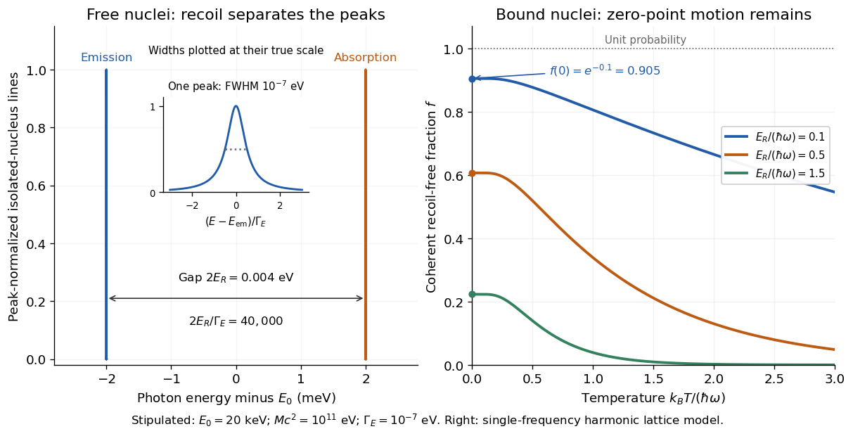
The Lamb-Mössbauer factor is the fraction in the coherent elastic line. In the harmonic-lattice approximation it is a Debye–Waller factor. Write the displacement of the emitting or absorbing atomic nucleus relative to its equilibrium site as , put , and define the angular wavenumber . Choose the equilibrium site so that . Its directional displacement variance is . A harmonic solid in thermal equilibrium has a Gaussian distribution for this displacement, whose characteristic function gives the elastic amplitudeTaking the squared magnitude gives the intensity fractionThe factor belongs to the amplitude exponent; it disappears when the amplitude is squared. For an isotropic solid, , so an equivalent expression is . Directional and three-dimensional mean squared displacements must not be substituted for one another without this factor.
An Einstein solid approximation replaces the vibrational spectrum by one positive angular frequency . For the directional quantum harmonic oscillator, with the same effective mass as in ,Here is the Boltzmann constant and is temperature. This follows by taking the expected value of in each oscillator energy eigenstate, , and averaging with the Boltzmann distribution. Substitution givesThe zero-temperature limit retains zero-point energy and a nonzero displacement variance. Cooling therefore increases the recoil-free fraction towards a limit below one for finite . At high temperature, the exponent tends to . This is a single-frequency approximation to a harmonic lattice's coherent elastic weight, not a complete description of all zero-net-energy processes of an isolated oscillator. Real vibrational spectra, directional binding and anharmonic motion can change its predictions.
Extend the stipulated teaching system by choosing , so . Then , while at . If source and absorber are independent, the fraction of events eligible for recoil-free emission followed by recoil-free absorption contains the product ; this gives for two zero-temperature copies. It is not the total probability of absorption, which also depends on the number of resonant atomic nuclei, geometry and spectral line overlap.
Acetone iodination rate-law experiment 2026-10-18
Acetone reacts with iodine to form iodoacetone, iodide, and a hydrogen ion:In water, denotes a solvated hydrogen ion; added hydrochloric acid provides acidic conditions.
Moorpark College's protocol mixes acetone, hydrochloric acid and water from burets in matched test tubes; pipet in iodine, swirl and time colour loss against white paper. Use water, then reacted solution, as references. Duplicate each mixture; keep total volume and run temperatures within .[ref]
Experiment 4: Chemical Kinetics: The Iodination of Acetone. Chemistry M01B Laboratory Manual, version 4.0 by Moorpark College Department of Chemistry; Version 4.0, Experiment 4, printed pp. 17–18: Procedure and Table 1
The stock dilutions give , , and . B and C separately double acetone and acid; D halves iodine. The manual supplies no measured times; it states zero partial order of reaction in iodine and asks students to determine the other exponents.[ref]
The endpoint measurement is a time to an operational colour threshold, not direct observation of a reaction intermediate. If the iodine disappearance rate is approximately constant until that endpoint, . Halving at fixed other concentrations then approximately halves without changing . A longer or shorter endpoint time alone is not a comparison of reaction rates unless the starting concentration is included. For an observed power-form rate law, doubling only acetone gives a rate ratio and hence ; doubling only acid similarly estimates its own partial order of reaction. Those are inference formulas, not asserted experimental results.
A useful proposed reaction mechanism would explain how iodine is consumed after an earlier transformation sets the throughput, making the observed reaction rate insensitive to iodine over a tested range. The observed zero exponent would contradict treating this net chemical equation as a single elementary reaction with directional rate law . It would not uniquely prove which reaction intermediate or earlier step is involved. Independently detecting a candidate reaction intermediate would provide another kind of evidence.
The excess-reactant approximation has an explicit scale: the baseline iodine inventory is only of the initial acetone inventory, and its net hydrogen ion production is of the initial acid inventory, assuming only the stated one-to-one chemical reaction. These are calculated bounds on composition change, not measured reaction orders. Mixing delay, a subjective colour threshold, and temperature drift limit the inference. Repeats and a fixed viewing geometry help; a calibrated absorbance trace could test linearity during conversion instead of relying on an endpoint alone. That extension would require a reference blank and a justified Beer-Lambert law calibration, rather than treating visible colour as an exact concentration. A zero-order reaction approximation in iodine must fail at depletion; it cannot imply consumption after no iodine remains.
Parallel first-order reaction mechanism 2026-10-18
A parallel first-order reaction mechanism consumes the same reactant through competing routes. Extend the product-split idea in catalytic selectivity by following both reaction products over time. Stipulate irreversible first-order reactions and in a uniformly mixed closed system of fixed volume and temperature. Initially only A is present, with concentration . With ,Here abbreviates a sum of rate constants, not an equilibrium constant. The rate equations are , , and . Integrating the last two after solving the first proves the expressions and their conserved total .
Choose two alternative models: model U has ; model V has . Both have , so every measurement of A alone is identical, even with no measurement error. Yet their P-to-Q concentration ratios at any are and , respectively. This is a precise failure of identifiability from that one observable. A calibrated measurement distinguishing P from Q resolves it within the stipulated two-route model.
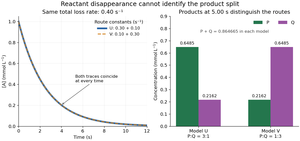


At , both models give . Model U gives ; model V exchanges these. Measuring only the summed reaction product concentration would also fail to distinguish them. Product-specific observations therefore answer a question that total conversion cannot. As with any reaction mechanism, fitting these observables still does not rule out a more elaborate untested route.
Consecutive first-order reaction mechanism Created 2026-10-18 Updated 2026-10-20
A consecutive first-order reaction mechanism passes material through a reaction intermediate. Consider a stipulated chemical reaction network , with constant positive rate constants, fixed temperature and volume, uniform mixing, and no reverse or competing chemical reactions. All three labels carry one conserved unit of material. Set and . The law of mass action givesAdding the three rate equations proves . Each step has a first-order reaction rate law; this does not make all three concentrations simple exponential decays.
For , the exact solution isTo derive the middle expression, substitute the first into the first-order linear differential equation for I and multiply by the integrating factor . Then , which can be integrated directly with the stated initial condition. The material balance supplies P without another integration.
The apparent division by zero at equal rate constants is removable. For , the same integrating factor givesThis is also the limit of the unequal-rate constant expression. Initially , so reaction product formation begins with zero slope despite immediate reactant loss. By contrast, a direct first-order reaction with the same has and nonzero initial slope. Their A traces agree exactly; their P traces do not.
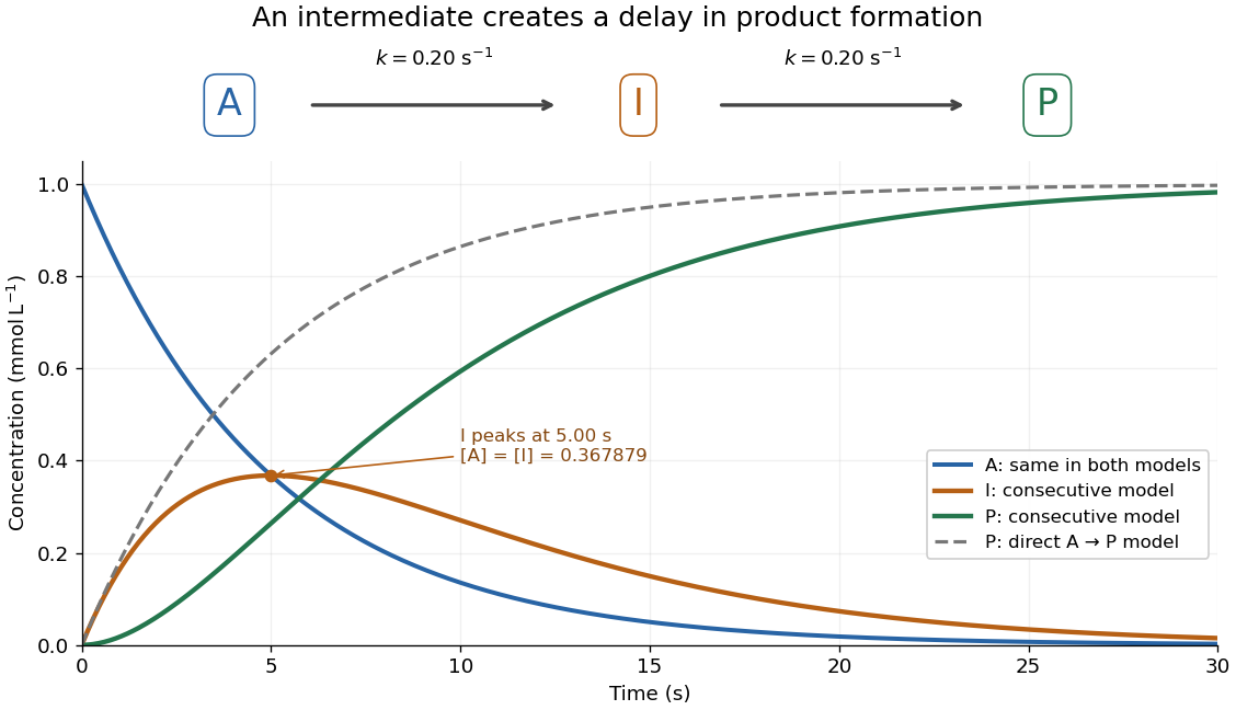
An accumulating reaction intermediate delays reaction product formation in a consecutive first-order reaction mechanism
. Original chosen model with and . Solid curves follow the exact three-species rate equations; the dashed P curve is a separate direct A-to-P model with the same A trace. These are model predictions, not measurements or an identified molecular reaction mechanism. Details.
For the chosen equal-rate constant example, I peaks at , because . At that time and ; the direct model would already have . The peak means formation and consumption of I are momentarily equal, not that the whole system has reached chemical equilibrium.
More generally the peak is at , which is positive for either ordering of the two positive rate constants and tends to as they coincide. When , a brief initial adjustment can be followed by and approximately equal formation and consumption reaction rates. The exact solution states when this small-intermediate approximation can be reasonable. It is inappropriate for the illustrated equal-rate constant case: at the peak, over one third of the conserved material is I. Such timing matters if the goal is to collect a useful reaction intermediate before it becomes the final reaction product.
Work by Raymond Webster Hayward 2026-10-18
Work by Raymond Davis Jr. 2026-10-18
There are unlisted articles, also show them or only show them.