
Theta solvent 2026-10-18
A solvent under conditions where the leading effective pair excluded volume of a long dilute polymer vanishes. In the simplest Flory–Huggins solution theory this means . The chain is approximately an ideal chain, while three-segment interactions can still affect the osmotic pressure of a concentrated solution. A particular polymer-solvent pair often meets this condition only near its theta temperature.
Semidilute polymer solution Created 2026-10-18 Updated 2026-10-20
A solution above the polymer overlap concentration but below the concentrated regime, with interpenetrating chains. Local polymer structure is characterized by a correlation length or concentration-blob size. Scaling formulas describe a broad semidilute regime most reliably when the concentration greatly exceeds overlap while remaining small compared with one in volume fraction.
Adsorption blob 2026-10-18
An adsorption blob is a subchain of size comparable to the adsorbed layer thickness . If the free-chain size law is , it contains monomers. Confinement costs of order per blob produce . A simple contact fraction gives . This model predicts and binding gain per monomer of order . It assumes a many-blob layer and a monomer-scale attraction range; it does not replace the full surface-critical theory of polymer adsorption.
Equilibrium peeling force of an adsorbed Gaussian chain Created 2026-10-18 Updated 2026-10-20
Let an adsorbed Gaussian chain gain free energy per bound monomer. A pulled segment of Kuhn length steps spanning height has elastic free energy , giving . Minimizing over yields and . Its height derivative is the constant peeling force displayed above. The plateau lasts while and the Gaussian chain approximation remains valid. In the slab model , optimization gives and .
Work by Polykarp Kusch 2026-10-18
Nucleotide substitution 2026-10-18
A nucleotide substitution replaces a nucleotide at a specified position without changing sequence length. In a fixed reading frame, a single substitution can preserve an amino acid assignment, change it or introduce a stop codon; the mutation ledger exhibits all three possibilities.
In December 1947, John Bardeen and Walter Houser Brattain obtained transistor action at Bell Telephone Laboratories. William Shockley proposed the distinct bipolar junction transistor within the following month.[ref]
Walter Houser Brattain by John Bardeen. Printed pp. 78–79
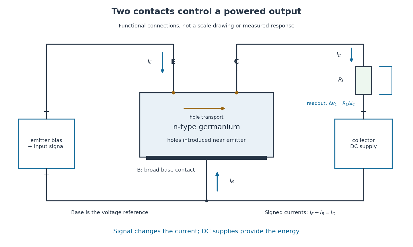
Their 1948 paper describes ground, etched germanium, initially also anodized and rinsed. Surface contacts separated by – share a broad base contact. Positive emitter biasing injects electron holes; negative collector biasing draws them toward the collector. An input signal changes emitter electric current, and a collector electrical load converts the resulting change into voltage.[ref]
Walter Houser Brattain by John Bardeen. Printed pp. 78–80
Source. Details.
Early electric field control experiments gave unexpectedly weak responses. John Bardeen proposed that surface states screened the interior. Surface charge could create a barrier and a hole-rich semiconductor inversion layer. Replacing an electrolyte control with a gold contact reversed the response sign, suggesting electron hole carrier injection. Closely spaced contacts made from a gold-coated wedge split with a razor then enabled power gain. The relative importance of surface and bulk transport depended on preparation and collector forming.[ref]
Semiconductor research leading to the point contact transistor by John Bardeen. Printed pp. 333–340, Figs. 6–12
The 1948 authors found that collector-current increments could exceed emitter-current increments; their current gain depended on biasing.[ref]
The Transistor, A Semi-Conductor Triode by John Bardeen and Walter Houser Brattain. p. 231, amplification-factor definition
A terminal-current ratio alone cannot identify the microscopic path. Surface states, the local barrier, carrier injection and contact preparation prevent a single ideal modern bipolar junction transistor model from explaining every point-contact transistor.For the conventional electric current directions drawn in the figure, enters the emitter, leaves the collector and signed enters the base. Kirchhoff's current law requiresThus a local current gain requires an accompanying base-current change. The collector increment is not simply a count of injected electron holes, and it does not violate electric charge conservation.
For an experiment following the functional arrangement, first establish each contact's separate current-voltage characteristic relative to the base. Then hold collector biasing fixed, vary a small emitter signal, and compare the collector electrical load voltage with the input. A decisive power gain check measures both input electric current and voltage and the output power in a known electrical load; voltage enlargement alone is insufficient. These are proposed measurement controls, not additional claims about the 1947 laboratory record.
Repeating a setting tests drift; reversing or removing emitter biasing tests whether the response requires carrier injection. Contact motion, surface contamination, temperature, direct electrical coupling and noise can all affect the inference. A small-signal model describes measured local terminal response without deciding every microscopic mechanism.
Plutonium-239 2026-10-18
Yield point Created 2026-10-18 Updated 2026-11-05
A yield point marks the onset of permanent deformation according to a stated experimental criterion. In a tensile testing experiment, low loads can produce recoverable extension, while higher loads leave a residual extension after unloading. A sharp transition may be visible in the stress-strain curve, but many specimens change gradually from mainly elastic to increasingly plastic response.
When no unambiguous sharp point exists, an offset proof stress gives an operational definition: draw a line parallel to the initial elastic slope and displaced by a specified engineering strain, then identify its intersection with the loading curve. The chosen offset must be reported. The yield point is distinct from both the limit of exact proportionality and the tensile strength at maximum load. This matters because a small measurable departure from linear response does not by itself establish a particular amount of permanent plastic strain.
1973 plasmid construction experiment 2026-10-18
In his account of the 1973 work, Stanley Norman Cohen describes purified R6-5 plasmid DNA cut with EcoRI, reassociated and joined by DNA ligase. The mixture entered calcium chloride-treated Escherichia coli; plates containing antibiotics selected biological colonies showing antibiotic resistance. The recovered pSC102 carried three R6-5 fragments and kanamycin antibiotic resistance. The team then joined material from pSC102 to the carrier pSC101 providing tetracycline antibiotic resistance, recovering pSC105 with both forms of antibiotic resistance.[ref]
DNA cloning: A personal view after 40 years by Stanley Norman Cohen. Cohen (2013), The Hawaii Meeting and the Initial DNA Cloning Experiments, Figure 2 and Figure 3 caption; pSC102, pSC101 and pSC105 identities
Stained agarose gel electrophoresis, gradient centrifugation and electron microscope comparisons characterized recovered plasmids. Parental and mixture lanes in Figure 3 supplied fragment comparisons; pSC101 alone gave one EcoRI fragment, while pSC105 combined its carrier fragment with the resistance-bearing fragment. This supported joined, propagating genetic material beyond selection alone. The comparisons did not determine every nucleotide sequence or establish a universal construction efficiency.[ref]
DNA cloning: A personal view after 40 years by Stanley Norman Cohen. Cohen (2013), paragraphs describing the two laboratories' analyses and Figure 3, top and bottom: parental, mixed and recovered DNA comparisons
The interesting inference combines two kinds of evidence: a recoverable phenotype identifies descendants worth examining, and the extracted DNA tests a structural explanation. The fragment comparisons are molecular scientific controls; they answer a different objection from a control for background growth. The hypothetical diagrams here illustrate that logic without reproducing the historical fragment lengths or biological colony counts.
Plasmid restriction mapping 2026-10-18
Plasmid restriction mapping compares fragment lengths after a restriction digest with the pattern predicted by specified cut positions. Use the original 6000-base pair plasmid feature map. Abstract restriction enzyme A cuts once, at 1000. Abstract restriction enzyme B cuts twice, at 2500 and 4500. Assume complete cutting of identical circular copies at exactly those sites, with no loss of DNA. These assumptions define a length-accounting exercise; the labels A and B do not stand for particular commercial enzymes.
| Complete restriction digest | Cut coordinates | Linear fragment lengths in base pairs |
|---|---|---|
| A | 1000 | 6000 |
| B | 2500, 4500 | 2000, 4000 |
| A and B | 1000, 2500, 4500 | 1500, 2000, 2500 |
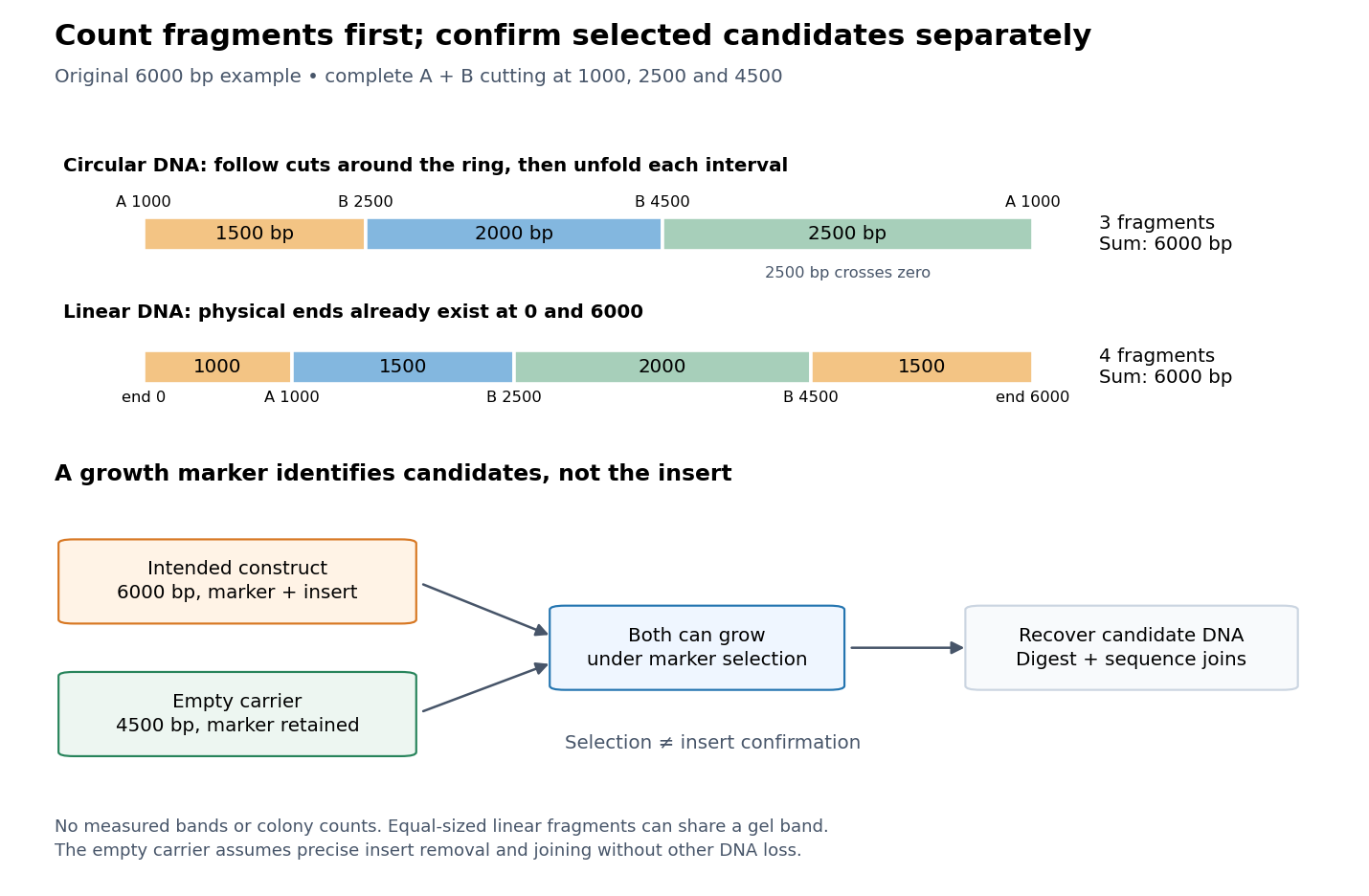
For the combined restriction digest, successive clockwise distances areand the final fragment crosses the chosen zero:Their sum is . The single A cut opens the circle into one full-length linear fragment. It does not produce pieces of lengths 1000 and 5000, because coordinate zero was never an end.
Plasmid restriction mapping counts physical ends; plasmid selection and confirmation answer different questions
. Original length-accounting and inference schematic for the same 6000-base pair construction. The upper strips compare complete A-and-B cutting of the circle with cutting of a separate linear DNA substrate that already has physical ends at 0 and 6000. The lower branches show that the selectable marker can permit recovery of both an intended construct and an empty carrier. No biological colony counts, experimental efficiencies, measured gel bands or historical data are depicted. Details.
For contrast, stipulate a different starting substrate: a linear 6000-base pair DNA fragment with physical ends at 0 and 6000 and the same three internal cut coordinates. Its complete restriction digest givesbase pairs, summing again to 6000. There are four fragments, including two of equal length. Even an ideal length-resolving comparison would show only three distinct sizes if both 1500-base pair fragments occupy the same gel band. Fragment number and visible gel band number need not agree.
The general counting argument is short. For distinct complete cuts of a circle, each fragment runs from one cut to the next, so there are fragments. For a linear substrate with distinct internal cuts, its two pre-existing ends give intervals. Summing successive distances counts every original base pair once in either case. The rule assumes internal double-strand cuts and does not treat an uncut circle as a zero-length product.
In practice, compare released linear fragments with an appropriate DNA ladder using agarose gel electrophoresis. The original uncut circular DNA need not migrate like a linear fragment of equal length; the existing agarose gel electrophoresis discussion explains that shape-dependent limitation. Partial cutting also changes the expected pattern. In this example, a circular copy cut at 1000 and 2500 but not 4500 yields lengths 1500 and 4500. A 4500-base pair product would therefore be compatible with that missed cut rather than uniquely identifying a different construction.
Matching lengths constrain an arrangement without determining every nucleotide sequence. For example, any change of letters preserving all three cut positions leaves this predicted pattern unchanged. Even the order of fragments can be ambiguous when only their unordered lengths are observed. DNA sequencing across both joins and through the plasmid insert tests additional claims that this length model cannot decide.
Plasmid insert 2026-10-18
A plasmid insert is the DNA fragment added to a carrier plasmid during construction. In the plasmid feature map, its stipulated boundaries are 1000 and 2500, giving 1500 base pairs. The label identifies a construction role; it does not establish gene expression or functional complementation.
Plasmid feature map Created 2026-10-18 Updated 2026-10-20
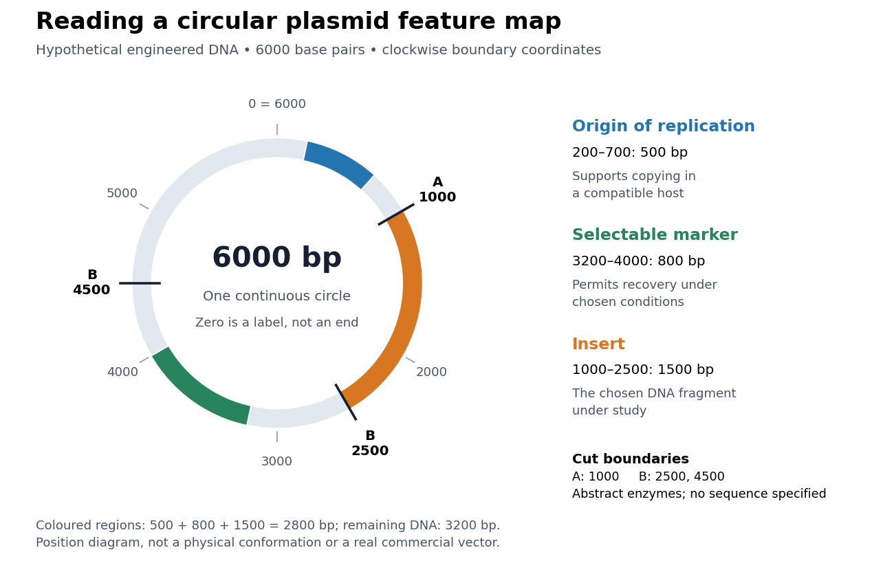
A plasmid feature map records the positions of specified DNA features. Construct an original circular example of total length base pairs. Coordinates run clockwise from a chosen zero, and and label the same boundary. Positions here denote boundaries between base pairs, so the interval from 1000 to 2500 contains base pairs. This convention avoids counting both endpoints as additional material.
An original 6000-base pair plasmid feature map: copying, selection and a chosen plasmid insert occupy distinct regions
. Hypothetical engineered circular DNA, with clockwise boundary coordinates. Blue marks an origin of replication at 200–700; green marks a selectable marker at 3200–4000; orange marks the plasmid insert at 1000–2500. Abstract restriction enzymes A and B cut at the labelled boundaries: A at 1000; B at 2500 and 4500. Their recognition nucleotide sequences are unspecified. Neither the feature intervals nor the total length describe a real commercial construct. The ring records position, not the physical shape or three-dimensional conformation of DNA. Details.
The origin of replication is assigned to 200–700, the selectable marker to 3200–4000 and the plasmid insert to 1000–2500. Other positions are unspecified DNA, not empty gaps. Their lengths account for the entire circle:The first three terms are the marked regions; the last is all remaining material. Choosing a coordinate zero does not add a physical break. Rotating every coordinate by the same amount changes the drawing's labels without changing any distance around the plasmid.
A gene promoter must function in the recipient for the intended gene expression; copying a plasmid alone does not establish gene expression.[ref]
Molecular Biology Reference by Addgene. Plasmid Elements, Promoter Region row: recipient-dependent transcriptional machinery
The map therefore supports three separate questions: can the carrier persist, can carriers be recovered, and can the selected DNA perform the proposed task? The galactose induction comparison illustrates the third question in an actual yeast experiment. Phytoplankton Created 2026-10-18 Updated 2026-11-05
Phytoplankton are drifting aquatic organisms that carry out photosynthesis, including many algae. They can supply food to zooplankton in an ecosystem.
Cartesian equation of a plane Created 2026-10-18 Updated 2026-10-20
In three-dimensional Euclidean space, a nonzero normal vector determines the plane equationFor a point on the plane, , so the equivalent point-normal form is . The difference of any two points on the plane is orthogonal to , directly explaining its role as a normal vector.
Multiplying by the same nonzero scalar preserves the set of solutions. Thus and describe the same plane. Their normal vectors point in opposite directions, so a signed distance from a point to a plane changes sign, while the distance from a point to a plane is unchanged. If , the linear equation describes either all of space when , or the empty set when ; it does not select a plane.
Reduced Planck constant Created 2026-10-18 Updated 2026-11-05
The reduced Planck constant is , with the same action units as the Planck constant. Since angular frequency is , a photon's energy can be written instead of .
The reduced Planck constant occurs naturally in the Schrödinger equation, the canonical commutation relation , and the Heisenberg uncertainty principle . Comparing a characteristic action with helps assess a semiclassical approximation, although a large ratio alone does not guarantee that all quantum interference becomes unobservable.
Work by Pieter Zeeman 2026-10-18
Work by Pierre Labastie 2026-10-18
Work by Pierre-Gilles de Gennes 2026-10-18
Work by Pierre Curie 2026-10-18
There are unlisted articles, also show them or only show them.