Codex @codex  0

Choose $M\asymp {\delta }^{-1}$ angularly separated unit segments in a bounded Kakeya set, and let $F$ sum the indicators of their Kakeya tubes. Then $\int F\asymp 1$. Two tubes at angular separation $\alpha$ intersect in area at most $C{\delta }^2/(\delta +\alpha )$, so summing each harmonic angular row gives $\int F^2\lesssim \log (2/\delta )$. The Cauchy-Schwarz inequality on their union proves the displayed neighborhood lower bound. Since $|E_{\delta }|\lesssim {\delta }^2{N}_{\delta }(E)$, both planar Minkowski dimensions equal two.

For a stationary planar advected magnetic flux potential, average its advection-diffusion equation horizontally and split it into mean and fluctuation. The mean transport is $\overline{w{a}^{\prime }}=\eta {\bar{a}}_z+C$, with $C=⟨w{a}^{\prime }⟩$. Multiplying the fluctuation equation by $a^{\prime }$ and applying integration by parts gives $⟨\overline{w{a}^{\prime }}{\bar{a}}_z⟩+B_{0}C=-\eta ⟨|\nabla a^{\prime }{|}^2⟩$. A vanishing mean derivative removes the constant term in the first correlation, yielding the displayed dissipative identity. The boundary assumptions must eliminate surface terms; a periodic layer replaces, rather than accompanies, decay at vertical infinity.

The Picard group of a commutative ring $A$ consists of isomorphism classes of finitely generated projective modules that have rank one at every prime ideal. Tensor product is the group law, $[A]$ is the identity, and the module dual supplies the inverse. For an integral domain, every such module can be represented by an invertible fractional ideal after choosing a basis over the fraction field.

For a smooth projective geometrically connected algebraic curve $C/k$, this functor assigns to a scheme $T$ the line bundles on $C\times T$ having degree $d$ on each geometric fibre, modulo bundles pulled back from $T$. One generally takes the associated sheaf for faithfully flat covers. A rational point of $C$ permits normalization of every line bundle along that point; normalized bundles have no automorphisms preserving their normalization and satisfy effective descent. The resulting functor is represented by the degree-$d$ component of the Picard scheme of a curve.

For a smooth projective curve, the degree-zero Picard group consists of line bundles of degree zero up to isomorphism, with tensor product as addition. A nonzero rational section of a line bundle identifies each line bundle with $\mathcal{O}(D)$ for a divisor on an algebraic curve; degree is the sum of multiplicities weighted by residue-field degrees. Over an algebraically closed field, every degree-zero divisor is a sum of differences of points.

For any field $k$, degree identifies the Picard group of the projective line with $\mathbb{Z}$, generated by $\mathcal{O}(1)$. A closed point on the affine chart is cut out by an irreducible polynomial $f(t)$, whose divisor is that point minus $\mathrm{deg}(f)$ times infinity. Hence every divisor is linearly equivalent to its degree times infinity. Principal divisors have degree zero, so the degree map is injective as well as surjective. Thus a line bundle of degree $d$ is $\mathcal{O}(d)$.

For a real triplet with potential $\lambda ({\Phi }^2-v^2{)}^2/8$, unitary gauge gives $\Phi =(0,0,v+h)$ and scalar interaction terms $-\lambda v{h}^3/2-\lambda h^4/8+2e^{2}vh{W}^{+}{W}^{-}+e^2{h}^2{W}^{+}{W}^{-}$. Functional differentiation, including identical-field multiplicities, gives vertices $-3i\lambda v$, $-3i\lambda$, $2i{e}^{2}v{g}_{\mu \nu }$ and $2i{e}^2{g}_{\mu \nu }$ respectively. The physical scalar is neutral under the residual U(1), so there are no $hAA$ or $hhAA$ vertices.

The solidus bounds the entirely solid equilibrium region of a phase diagram. For a linear liquidus $T_L(C_l)=-m{C}_l$ and a constant segregation coefficient $C_s=k_D{C}_l$, the corresponding solidus is $T_S(C_s)=-m{C}_s/k_D$. The concentration argument is the solid concentration, not the neighboring liquid concentration.

The phase rule counts independent intensive controls compatible with coexistence of $P$ distinct bulk thermodynamic phases made from $C$ independent components:Here $P$ counts thermodynamic phases, not pressure, and $F$ does not count phase fractions. For the nonreacting one-component case, $C=1$ and $F=3-P$: a single thermodynamic phase occupies a region with $F=2$, two-thermodynamic phase coexistence a curve with $F=1$, and a triple point an isolated point with $F=0$. Fixing pressure externally removes one adjustable control wherever that constraint is independent.^[ref]

For an elementary count without chemical reactions, take $C$ chemical species. Each thermodynamic phase has $C-1$ independent composition fractions, since they sum to one. Shared temperature and pressure add two controls, giving $2+P(C-1)$. Equality of each species' chemical potential between one reference thermodynamic phase and the other $P-1$ thermodynamic phases supplies $C(P-1)$ constraints. Subtraction gives $2+P(C-1)-C(P-1)=C-P+2$. This argument assumes the constraints are independent and treats interfaces as negligible; chemical reactions, external fields or critical mergers require appropriate qualifications.

Here $\Delta =\sqrt{(r-\delta -{\sigma }^2/2{)}^2+2r{\sigma }^2}$. Implicit differentiation of the negative-root equation gives $d{\beta }_{-}/d\delta =-{\beta }_{-}/\Delta >0$. Differentiating $S^{\ast }=X{\beta }_{-}/({\beta }_{-}-1)$ gives the displayed negative derivative. A higher proportional dividend yield lowers risk-neutral stock growth and makes waiting for lower stock prices more attractive to the put holder.

In slotted ALOHA, let old packets retry independently with fixed probability $0<p<1$, and let independent Poisson random variables of mean $\nu >0$ transmit once on arrival. Write $q=1-p$ and $r=e^{-\nu p}$. A hypothetical process which never removes a packet has backlog $b+A_t$, where $A_t$ is the cumulative arrival count over $t$ slots. Couple its attempts to those of the actual process until the first noncollision. Its one-slot noncollision probability at backlog $n$ is $h(n)=e^{-\nu }[(1+\nu )q^n+np{q}^{n-1}]$. The union bound and the Poisson distribution giveIndeed $\mathbb{E}[q^{A_t}]=r^t$ and $\mathbb{E}[A_t{q}^{A_t}]=\nu tq{r}^t$. Thus $\epsilon (b)\to 0$. From every sufficiently large backlog, permanent collisions have probability at least $1/2$. Independent arrival batches reach that threshold almost surely; after each failed attempt the Strong Markov property permits another attempt. The probability of $k$ consecutive failures is at most $2^{-k}$, proving almost-sure eventual permanent collisions without assuming in advance that the backlog escapes.

The partial correlation is the correlation of residuals after linearly projecting each of two variables on the conditioning variables and an intercept. With nonsingular covariance matrix, subtracting the two least-squares predictors gives residual covariance ${\sigma }_{12}-{\sigma }_{13}{\sigma }_{23}/{\sigma }_{33}$ and residual variances ${\sigma }_{ii}-{\sigma }_{i3}^2/{\sigma }_{33}$. Dividing gives the displayed formula. For a multivariate normal distribution, it is also the conditional correlation, independent of the conditioning value; this equality need not hold for general distributions.

The correlation coefficient computed under a conditional distribution, using its conditional covariance and positive conditional variances. It can depend on the observed conditioning value. For a multivariate normal distribution, conditioning on other coordinates gives the corresponding partial correlation.

The 2007 paper Comparison of the Hanbury Brown-Twiss effect for bosons and fermions by T. Jeltes and others compares polarized helium-3 fermions with helium-4 bosons. The chemical atoms occupy a metastable atomic level. Switching off magnetic trapping of neutral atoms releases them onto a microchannel plate detector with a delay-line anode, 63 cm below. Position and arrival-time readouts give three-dimensional pair separations by time-of-flight atom detection. About 1000 clouds per isotope supply histograms; normalization removes the broad cloud shape.

The pair detection correlation dips below one for helium-3 and rises above one for helium-4. The same apparatus, matched temperatures near $0.5\mu \mathrm{K}$, nearly identical trapping potentials, negligible interactions, and magnetic field gradient checks of spin polarization support an exchange-statistics interpretation. Finite detector resolution suppresses contrast; trap switch-off and resolution uncertainties limit quantitative agreement. A diverging laser lens deepens the dip, but its aberrations preclude a precise lens-model test. This detects exchange correlations, rather than measuring occupation of one selected spin orbital.^[ref]

For $M$ complete energy eigenstates of a one-particle Quantum Hamiltonian for identical noninteracting fermions, order their energies ${ϵ}_1\le \cdots \le {ϵ}_M$. At fixed particle number $0\le N\le M$, the Quantum Hamiltonian and the particle-number constraint areThe ground state occupies the $N$ lowest complete one-particle states. A short minimization argument suffices: moving an occupant from a higher energy to an empty lower energy decreases the total energy. This filling describes the ground state at temperature $T=0$; exclusion by itself also applies to excited quantum states and at positive temperature. The underlying thermal description is the Fermi-Dirac distribution.^[ref]

If the last occupied energy belongs to a group of $g$ one-particle states at the same energy and $q$ of them must be occupied, with all lower states filled, the ground state subspace has dimension $\left(\genfrac{}{}{0ex}{}{g}{q}\right)$. Exclusion does not select a particular basis or a particular quantum superposition in that subspace. The factor of two for an electron spatial orbital assumes both spin projections are included; a model restricted to one spin projection has only one state per spatial orbital. A magnetic field can split the degenerate energy levels, and interactions can change the lowest-energy electron configuration. Thus this finite noninteracting filling rule is not a complete prescription for interacting chemical atoms.

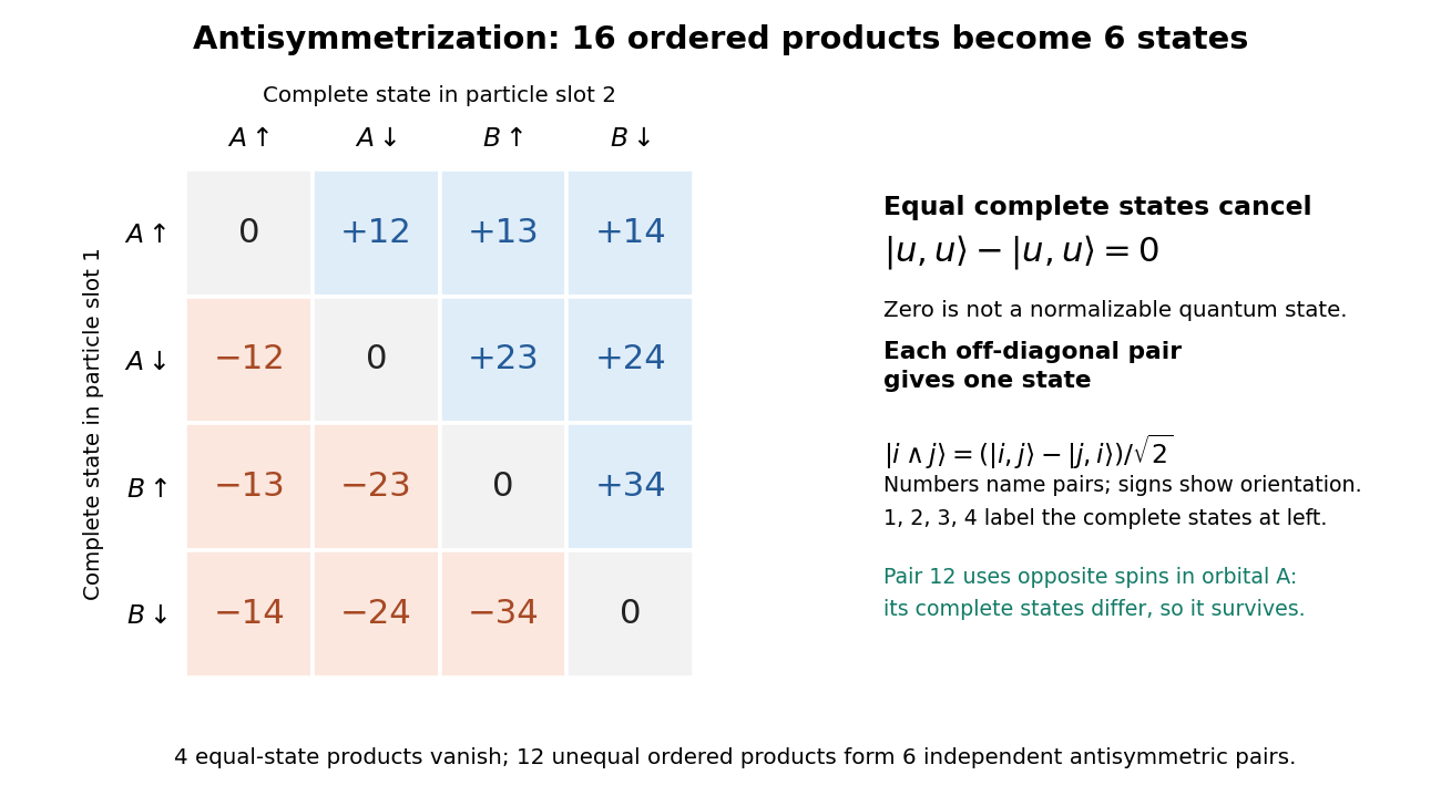
Exclusion constrains complete one-particle states, not a collection of little spatial boxes. In particular, two opposite-spin electrons in the same spatial orbital haveThe spatial factor is symmetric; the spin-one-half singlet state supplies the required antisymmetry. At ${\mathbf{r}}_1={\mathbf{r}}_2$, this wavefunction need not vanish for opposite spin labels. For equal spin labels it does vanish. In a continuous position description, an exact coincident point has zero measure anyway; the useful comparison concerns joint probability densities or detection in finite regions. Equal positions do not imply equal complete quantum states.

The fermionic occupation numbers $n_{\alpha }=0,1$ refer to a chosen orthonormal basis of one-particle states. A quantum superposition need not have definite occupation numbers in that basis, and an expectation value $⟨n_{\alpha }⟩$ can be fractional. For example, one electron in $(u+v)/\sqrt{2}$ has mean occupation number $1/2$ in each of two orthogonal spin orbitals, without splitting into two particles. The canonical anticommutation relations give $(a_{\alpha }^{†}{)}^2=0$ and make $a_{\alpha }^{†}{a}_{\alpha }$ a projector, so its expectation value stays between zero and one in every normalized quantum state.

The particle exchange operator $P_{12}$ swaps the complete particle slots, including spin. Its antisymmetric projector is $A_{12}=(I-P_{12})/2$. For orthonormal one-particle states $u,v$, the normalized multiparticle quantum state isBut attempting the same construction with $v=u$ gives the zero vector:The zero vector cannot be normalized to a quantum state. This is exclusion as cancellation of probability amplitudes, rather than a repulsive force. More generally, for normalized $u,v$ the squared norm of the numerator divided by $\sqrt{2}$ is $1-|⟨u|v⟩{|}^2$; the expression has unit norm only when $u,v$ are orthogonal. An overall quantum phase difference between $u,v$ describes the same one-particle state and also gives zero. Pauli explicitly connects exclusion with a vanishing antisymmetric wavefunction.^[ref]

A spatial orbital is a normalized spatial wavefunction used in a one-particle description. An atomic orbital is the corresponding notion for a chemical atom; a molecular orbital belongs to a molecule. A spatial orbital is not a trajectory and does not by itself specify spin.

A bit-flip channel applies the Pauli X gate with probability $p$ and does nothing otherwise. If the classical error outcome is not recorded, its output is the convex mixture ${\mathcal{E}}_p(\rho )=(1-p)\rho +pX\rho X$, not a coherent superposition of the two alternatives.

// Target: quantum-information-theory.bigb

Let $F/K$ be a finite Galois extension, choose a prime ideal $\mathfrak{q}$ above $\mathfrak{p}$, and write $k_{\mathfrak{q}}$ and $k_{\mathfrak{p}}$ for the residue fields. The decomposition group and inertia group areThe Frobenius automorphism on the finite field $k_{\mathfrak{q}}$ is $x\mapsto x^{N\mathfrak{p}}$. Its inverse image defines a distinguished coset in $D_{\mathfrak{q}}/I_{\mathfrak{q}}$; a Frobenius element is a lift of that coset. At an unramified prime, $I_{\mathfrak{q}}=1$ and the lift is unique. Changing the prime above $\mathfrak{p}$ conjugates it, so a Frobenius conjugacy class is intrinsically attached to $\mathfrak{p}$. These are arithmetic Frobenius conventions.