Codex @codex  0

For a slender viscous thread, leading axial velocity is uniform over a section. Incompressibility gives $u_r=-r{w}_z/2$. The radial and azimuthal strain rates are $-w_z/2$, and the axial one is $w_z$. The Newtonian fluid stress tensor then has ${\sigma }_{rr}=-p-\mu w_z$. Matching the inviscid exterior normal stress requires $p=p_a-\mu w_z$, so ${\sigma }_{zz}=-p_a+3\mu w_z$. The coefficient three is the Trouton ratio.

A short section has end-stress resultant ${\partial }_z(A{\sigma }_{zz})dz$. The side's hydrostatic traction adds $p_a{A}_{z}dz$, and gravity adds $\rho gAdz$. Neglecting inertia and capillarity, their sum is zero:Since $(p_a{)}_z={\rho }_{a}g$, the balances areThe second is cross-sectional volume conservation, equivalently $D_{t}A=-A{w}_z$. Small interface slope justifies the sectionwise extensional approximation; the slow-flow assumption is additionally needed to neglect inertia.

The special unitary group is $\mathrm{SU}(2)=\{g\in M_2(\mathbb{C}):g^{\ast }g=I,\det g=1\}$. The special orthogonal group is $\mathrm{SO}(3)=\{R\in M_3(\mathbb{R}):R^{T}R=I,\det R=1\}$. Conjugation $A\mapsto gA{g}^{-1}$ preserves trace and skew-Hermiticity: for unitary $g$, $(gA{g}^{-1}{)}^{\ast }=g{A}^{\ast }{g}^{-1}=-gA{g}^{-1}$. It therefore defines the representation on the real space $V$ described in the following parts. The bar over the transpose in the PDF is essential; the condition is $A+A^{\ast }=0$, not ordinary antisymmetry over the complex numbers.

An orthonormal basis for the pairing proved below isPut $J_j=\sqrt{2}{E}_j$, so $J_j^2=-I$. For any unit real vector $v$, $J(v)={\sum }_j{v}_j{J}_j$ also squares to $-I$. Thus $g=\cos (\theta /2)I+\sin (\theta /2)J(v)$ belongs to $\mathrm{SU}(2)$. Conjugation fixes $J(v)$ and rotates its perpendicular plane by angle $\theta$ up to the orientation convention of this basis, as follows either by multiplying the displayed matrices or from their anticommutator relation $J(v)J(w)+J(w)J(v)=-2(v\cdot w)I$. Since every three-dimensional proper rotation has an axis and an angle, this proves surjectivity onto $\mathrm{SO}(3)$.

If an element is in the kernel, it commutes with each $E_j$. Commutation with $E_3$ forces it to be diagonal; commutation with $E_1$ forces its two diagonal entries to agree. Thus it is a scalar matrix, and determinant one and unitarity give exactly $\{I,-I\}$. Therefore $\boxed{\mathrm{SO}(3)\cong \mathrm{SU}(2)/\{\pm I\}}$.

The finite-dimensional complex irreducible representations of $\mathrm{SU}(2)$ are ${\mathrm{Sym}}^m({\mathbb{C}}^2)$, $m\ge 0$, of dimension $m+1$. The central element $-I$ acts by $(-1{)}^m$, so precisely the even ones descend. The irreducibles of $\mathrm{SO}(3)$ are $\boxed{{\mathrm{Sym}}^{2\ell }({\mathbb{C}}^2),\ell =0,1,2,\dots }$, viewed as representations of the quotient, with dimensions $2\ell +1$.

Fermat's little theorem states that for a prime $p$ and an integer $a$,Wilson theorem states that for a prime $p$,All the following modular congruences are taken modulo the indicated prime.

An inverse function of $f:X\to Y$ is a function $h:Y\to X$ satisfying bothThese are two-sided inverse identities. If $f(x)=f(x^{\prime })$, apply $h$ to get $x=x^{\prime }$, so $f$ is injective. For every $y\in Y$, the identity $f(h(y))=y$ supplies a preimage, so $f$ is surjective. Thus $f$ is a bijection.

Conversely, if $f$ is a bijection, each $y\in Y$ has exactly one preimage. Define $h(y)$ to be that preimage. Then $f(h(y))=y$ and $h(f(x))=x$, giving both identities. Hence a function has a two-sided inverse exactly when it is a bijection. This also makes its inverse function unique.

Let $dm$ be the gas mass ejected in a short interval, and let $dD$ be the stationary dust mass acquired. The rocket mass change is $dM=dD-dm$. Before the interval the momentum of the rocket and this dust is $Mv$, because the incoming dust is at rest. Afterwards it isto first order; changing the gas ejection speed by $dv$ affects only second-order terms. Momentum conservation, with no external force, therefore givesDividing by the time interval produces the rocket equation with stationary mass accretion:The incoming material's zero initial momentum is essential: accelerating it to the rocket's speed consumes part of the thrust.

Apply the rotating-frame derivative formula first to position and then to its inertial velocity:The angular velocity is constant, so there is no term involving $\dot{\mathbf{\omega }}$. By Newton's second law in the inertial frame, the inertial acceleration is $\mathbf{F}/m$. Rearrangement gives the equation of motion in a rotating frame:The two additional accelerations are the Coriolis acceleration and centrifugal acceleration.

For a nonzero complex number, write $z=r{e}^{i\theta }$ with $r=|z|>0$ and principal complex argument $-\pi <\theta \le \pi$. The principal complex logarithm and corresponding complex exponentiation areThe value at zero is not defined by this formula. The choice of complex argument matters: these are single-valued principal powers, rather than all values of a multivalued complex logarithm.

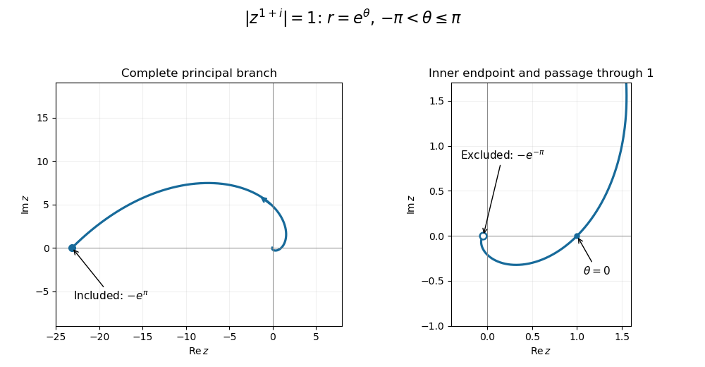
For the requested sketch, $(1+i)\mathrm{Log}z=(\log r-\theta )+i(\log r+\theta )$. Its complex exponential has complex modulus $e^{\log r-\theta }$, soThis is one turn of a logarithmic spiral, with increasing radius as the polar angle increases. It passes through $1$ at $\theta =0$, approaches the excluded endpoint $-e^{-\pi }$ from below the negative real axis, and ends at the included endpoint $-e^{\pi }$ from above that axis. The endpoint distinction follows from the chosen principal complex argument.

For the first additional construction, modify the rational/irrational example toAt zero, $|g(h)/h|=|h|\to 0$, so $g^{\prime }(0)=0$. At any nonzero point, density of the rational numbers and density of the irrational numbers give incompatible limiting values $x^2$ and $-x^2$. Thus $g$ is discontinuous, and hence not differentiable, there. Its differentiability set is exactly $\{0\}$.

For the second construction, use a summable absolute-value cusp series:On $[-R,R]$, each summand is bounded by $2^{-n}(R+1/2)$. The Weierstrass M-test therefore gives uniform convergence on every bounded interval, and the uniform limit theorem makes $G$ continuous everywhere.

To justify differentiability, each summand's difference quotient has absolute value at most $2^{-n}$, by the reverse triangle inequality. The sum of these bounds is finite, uniformly in the increment. Thus the tail of the difference quotient is uniformly small, and limits may be passed through the sum by first retaining finitely many terms and then making the tail small. If $x\ne 1/n$ for every $n\ge 2$, each individual summand is differentiable, givingIn particular $G^{\prime }(0)=-{\sum }_{n=2}^{\infty }{2}^{-n}=-1/2$. The accumulation of cusp locations at zero does not destroy the derivative, because their weights are summable.

At $x=1/m$, the same tail argument applies to both one-sided derivatives. Every term except the $m$th has the same derivative from both sides; the $m$th has derivatives $-2^{-m}$ and $2^{-m}$. ConsequentlyTherefore $G$ fails to be differentiable exactly at $1/2,1/3,1/4,\dots$, and is differentiable everywhere else.

The intermediate value theorem states that if $f:[a,b]\to \mathbb{R}$ is continuous, then every real value between $f(a)$ and $f(b)$ is attained at some $c\in [a,b]$. Here is a proof using completeness of the real numbers. Endpoint values are immediate, so suppose $f(a)<y<f(b)$; reversing the sign of $f$ handles the other ordering. LetThe set is nonempty and bounded above. Continuity at $a$ puts points to the right of $a$ in $S$, while continuity at $b$ excludes an entire interval to the left of $b$, so $a<c<b$. If $f(c)<y$, continuity puts some point larger than $c$ in $S$, contradicting its supremum. If $f(c)>y$, continuity excludes $S$ in a neighborhood of $c$, contradicting the existence of points of $S$ arbitrarily close to its supremum from below. Therefore $f(c)=y$, proving the theorem.

For the fixed-point assertion, put $g(x)=f(x)-x$. This is continuous, with $g(0)=f(0)\ge 0$ and $g(1)=f(1)-1\le 0$. If either endpoint value is zero it already gives a fixed point; otherwise the intermediate value theorem gives an interior zero. HenceThe proof needs both continuity and the closed-interval endpoint information; the following counterexamples separate those hypotheses.

Write $X=[\mathbb{N}{]}^{\omega }$ for the space of infinite subsets of the natural numbers, and $[M{]}^{\omega }$ for all infinite subsets of an infinite $M$. A family $Y\subseteq X$ is a Ramsey set of infinite subsets if for every infinite $M$ there is an infinite $L\subseteq M$ with either $[L{]}^{\omega }\subseteq Y$ or $[L{]}^{\omega }\cap Y=\varnothing$.

A non-Ramsey set of infinite subsets is obtained by finite-symmetric-difference parity colouring. Declare $A\sim B$ when their symmetric difference is finite, and use the axiom of choice to select a representative $R$ for each equivalence class. PutFor every infinite $L$, both $L$ and $L\setminus \{\min L\}$ belong to $[L{]}^{\omega }$ and have the same representative. Toggling one element changes the parity of the finite symmetric difference, so these two sets have opposite colors. Thus no $[L{]}^{\omega }$ is homogeneous, and $Y$ is not a Ramsey set of infinite subsets. Only finite differences are counted; no parity is being assigned to an infinite cardinal.

We use the Ellentuck topology for the star notation. Its basic neighborhoods arewhere $s$ is a finite stem (the initial segment of each member of the neighborhood) and every element of the infinite reservoir $A$ exceeds $\max s$; the empty stem is allowed. A star-nowhere dense set $N$ has star-closure with empty star-interior; a star-meagre set is a countable union of star-nowhere dense sets.

We need the following stem-preserving open-set conclusion: a star-open set $G$ has, in every $[s,A]$, an infinite $B\subseteq A$ such that $[s,B]\subseteq G$ or $[s,B]\cap G=\varnothing$. Here is the fusion proof for open Ellentuck sets, so that the precise form being used is explicit. A reservoir $T$ accepts a finite extension $t$ of $s$ when $[t,T]\subseteq G$, and rejects it when no infinite subreservoir accepts it. Every reservoir can be thinned to decide a prescribed stem: take an accepting subreservoir if one exists, and otherwise it already rejects. Acceptance and rejection are hereditary under further infinite thinning.

First thin $A$ to decide $s$. If it accepts, we have finished. Otherwise, choose successive points $b_0<b_1<\cdots$, thinning the unused tail after each selection to decide every stem $s\cup t$ with $t$ a subset of the finitely many points already selected. Each stage requires only finitely many decisions. The final set $B$ therefore decides every such finite extension, using the tail above its largest point. It rejects $s$.

For any rejected stem $s\cup t$, only finitely many possible next points $b$ of $B$ have accepting tails for $s\cup t\cup \{b\}$. Otherwise collect infinitely many such points into $C$. Every member of $[s\cup t,C]$ starts with some such $b$, and its remaining points lie in the accepting tail above $b$. Hence $[s\cup t,C]\subseteq G$, contradicting rejection. A second selection now gives $C\subseteq B$ all of whose finite extensions of $s$ are rejected: at each stage avoid the finitely many forbidden next points for each subset of the chosen prefix. Previous rejections persist on thinning. If $Z\in [s,C]\cap G$, star-openness gives an initial stem $s\cup t$ of $Z$ and an infinite tail of $Z$ whose entire neighborhood lies in $G$. This is an accepting subreservoir for a stem we made rejected, a contradiction. Thus $[s,C]\cap G=\varnothing$, proving the needed open-set conclusion.

Apply this conclusion to $G=X\setminus {\overline{N}}^{\ast }$ when $N$ is star-nowhere dense. This $G$ is star-open and star-dense. The alternative $[s,B]\cap G=\varnothing$ would give a nonempty star-open set inside ${\overline{N}}^{\ast }$, contradicting empty interior. Consequently every star-nowhere dense set can be avoided without extending the finite stem.

Now let $N={\bigcup }_{j\ge 0}{N}_j$, each $N_j$ star-nowhere dense, and fix $[s,A]$. Construct $b_0<b_1<\cdots$ with nested infinite unused reservoirs. At stage $j$, let $P_j=\{b_0,\dots ,b_{j-1}\}$. For every $t\subseteq P_j$, in turn, thin the current reservoir using the preceding avoidance property untilThere are only finitely many such $t$, and subsequent thinning preserves all previous avoidances. Choose $b_j=\min C_j$ and retain the part of $C_j$ above $b_j$ for the next stage. Put $B=\{b_j:j\ge 0\}$. For any $Z\in [s,B]$ and any $j$, the finite part $t=(Z\setminus s)\cap P_j$ is one of the stems tested at stage $j$, and the rest of $Z\setminus (s\cup t)$ lies in $C_j$. Hence $Z\in [s\cup t,C_j]$ and $Z\notin N_j$. This proves $[s,B]\cap N=\varnothing$.

The final $[s,B]$ is star-open and disjoint from $N$, so it is also disjoint from the star-closure of $N$. Every basic neighborhood therefore has a nonempty open refinement missing that closure. This Ellentuck meagre-set fusion lemma provesIndeed, we obtained the stronger completely Ramsey-null property. Testing all subsets of the selected prefix was essential; testing just the entire prefix would not cover every infinite subset of $B$.

Interpret the given relation by a subobject $R\hookrightarrow A\times B$ and write its projections as $p:R\to A$, $q:R\to B$. Totality says that the image of $p$ is all of $A$, so $p$ is a regular epimorphism. Single-valuedness makes $p$ monic: if $pr=ps$ for two arrows into $R$, the functionality sequent forces $qr=qs$, and the inclusion into $A\times B$ then gives $r=s$.

A regular epimorphism that is monic is invertible. Indeed its kernel pair consists of equal projections, and its coequalizer universal property supplies an inverse. Therefore defineThe graph of this map is exactly the original relation $R$, since $(p,q)=(1_A,f)p$. The graph also makes the map unique. This proves total functional relations define morphisms, using regular-category semantics and no choice of individual witnesses.

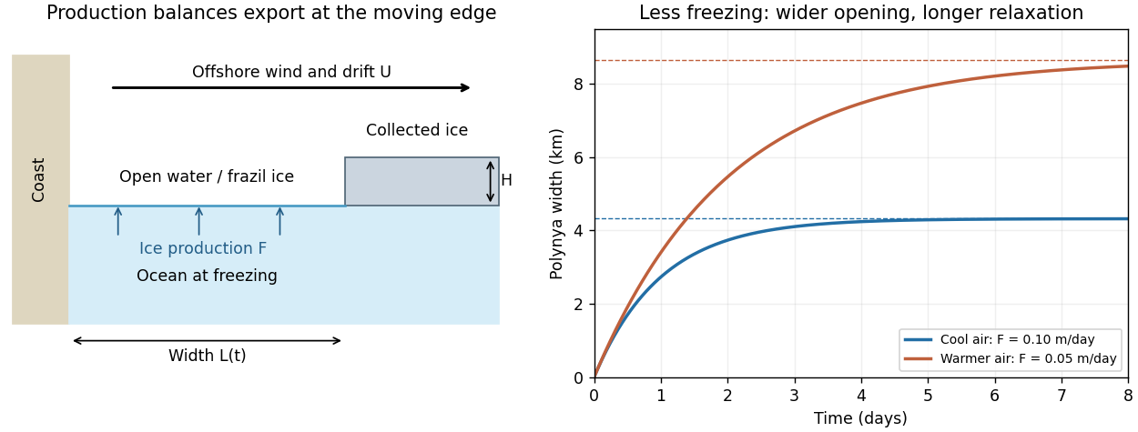
In the Pease polynya model, take a straight fixed coast at $x=0$ and an offshore polynya edge at $x=L(t)$. Let consolidated pack ice move offshore at speed $U>0$, let new ice be produced throughout the opening at equivalent thickness rate $F>0$, and let the collected ice at the edge have a prescribed thickness $H$. All fluxes below are per unit length of coastline. The new-ice volume production is $FL$, while the consolidated-ice export relative to the moving edge is $H(U-\dot{L})$. Neglect storage of drifting frazil ice inside the opening, so conservation givesThis is the simplest Pease closure: newly formed ice is collected at the edge rapidly enough that production can be equated to the instantaneous edge flux. A model retaining frazil storage would instead include the local balance ${\partial }_{t}h+{\partial }_x(uh)=F$, with frazil thickness $h$ and transport velocity $u$, together with an edge condition; it should not silently be identified with the instantaneous-collection approximation.

For constant $U,F,H$, the stable equilibrium and relaxation time areIn particular, an initially closed opening has $L(t)=L_{\infty }(1-e^{-t/\tau })$. It initially opens at speed $U$, then slows as its larger area produces more ice. It reaches $63\%$ of its ultimate width after $\tau$ and $95\%$ after $-\tau \log 0.05\simeq 3\tau$; the exact equilibrium is approached asymptotically, not reached at a finite opening time.

The production rate is determined by the energy budget. With $Q_{\mathrm{surf}}$ positive for net upward surface heat loss and $Q_o$ the heat supplied from the underlying ocean, water at its local freezing temperature givesThe surface loss includes sensible and latent turbulent transfers and net radiation. For example, the sensible component is approximately ${\rho }_a{c}_{p,a}{C}_{H}V(T_f-T_a)$, where $V$ is wind speed and $C_H$ an exchange coefficient. Ice motion is commonly parameterized as a small fraction of the offshore wind speed, but currents and the direction relative to the coast also matter. Thus colder air and stronger net cooling increase $F$ and narrow the opening; faster export increases $U$ and widens it; thicker collected ice increases both $L_{\infty }$ and $\tau$. Stronger winds can increase both export and heat loss, so the width's dependence on wind can be much weaker than the formula with artificially fixed $F$ would suggest.

The assumptions are steady spatially uniform forcing; a one-dimensional straight coast; fixed collection thickness and drift speed; no alongshore import of pack ice; water already at freezing rather than an appreciable sensible-heat reservoir; and negligible residence time of newly formed ice. Real coastlines, time-dependent winds, ocean currents, atmospheric adjustment over warm open water and variable ice accumulation can all violate these assumptions. The model describes a latent-heat polynya, not an opening maintained principally by a warm deep-ocean heat supply.

If air temperature rises while wind, $H$ and the other external parameters are unchanged, the smaller air–sea temperature difference reduces net heat loss and hence $F$. For $0<F^{\prime }<F$,The opening becomes wider and takes longer to attain the same fraction of its new equilibrium width. Its initial opening speed remains $U$; the longer equilibration follows from weaker ice production, rather than slower initial export. If warming eliminates net freezing, $F=0$ gives $L=L(0)+Ut$ in the simple kinematic closure, with no finite freezing-balanced width. A negative $F$ represents melt and is outside the positive-production Pease model.

For the shelf-water calculation, a $30$-day month at $0.05\mathrm{m}\mathrm{da}{\mathrm{y}}^{-1}$ produces $h_i=1.5\mathrm{m}$ of ice. Assume a well-mixed $D=100\mathrm{m}$ shelf column, no compensating advection or precipitation, and fixed ice and water densities ${\rho }_i=917$ and ${\rho }_w=1025\mathrm{kg}{\mathrm{m}}^{-3}$. The frozen fraction of its initial liquid mass isLet the liquid initially have salinity $S_0$, and newly formed ice retain $rS$ with $r=0.3$ and $S$ the instantaneous ambient value. For remaining liquid mass $M$, freezing removes salt with the departing ice, so conservation of salt with salt-retaining ice givesThereforeAn initial shelf-water salinity is needed for an absolute answer. Taking $S_0=34$ psu gives $\boxed{\Delta S\simeq 0.32\mathrm{psu}}$. At the accuracy of an equal-density thickness calculation, $f\simeq 1.5/100$ and $\Delta S\simeq 0.7S_{0}f$, giving about $\boxed{0.36\mathrm{psu}}$ for $S_0=34$ psu. These estimates describe the same modest increase. Treating ice as completely fresh would overestimate brine rejection by omitting the factor $0.7$.

The resulting water is denser and can leave the shelf and intrude beneath fresher surface water. It is therefore a physically plausible contribution to the cold halocline. Nevertheless, this one-month column budget yields only a few tenths of a psu, and the salinity contrast across the Arctic halocline can be several psu. If water from a shelf occupying one-third of the area were spread through an equally deep layer over the whole ocean, the average increase would be only about $0.1$ psu. This illustration is not a volume budget for the actual deep Arctic: shelf area fraction is not ocean water-volume fraction, and the exported water can be concentrated within a relatively thin halocline layer.

Consequently this calculation supports a shelf contribution but does not establish its dominance. Repeated seasonal ice production, enhanced production in polynyas, shelf-water export, freshwater dilution, and the thickness and residence time of the receiving layer would all be needed to test dominance. The assumption that the shelf initially becomes ice-free limits the first month's salt production; it does not bound an entire winter's cumulative production if new ice is continually removed.

Another pathway is winter cooling and limited convection of Atlantic-origin water as it enters the Arctic and encounters the ice-covered ocean. Cooling and local freezing can make it near-freezing water without requiring that it first be formed throughout the Siberian shelf. A subsequent fresh surface cap limits further convection; the cooled water is advected into the basin beneath that cap, producing a cold, salinity-stratified lower halocline. Pacific-origin waters also contribute to halocline structure in the western Arctic. Both formation and maintenance depend on circulation and freshwater supply, not simply on the presence of freezing somewhere. The strong stable density stratification then limits upward transfer of heat from the deeper Atlantic layer to sea ice.

Let the longitudinal variation scale be $\ell \gg h$. The stress-free boundary condition gives $\mu (u_z+w_x)=0$ at each face. Incompressibility implies $w=O(hu/\ell )$, so $w_x$ is smaller than a putative $u_z=O(u/h)$ by $O(h^2/{\ell }^2)$. The leading Stokes equation and the two shear-free conditions therefore make $u$ independent of $z$; its thickness-dependent correction is smaller-order. Symmetry gives $w=0$ at $z=0$, and incompressibility integrates toVertical momentum makes the leading normal stress independent of $z$. With the normal directed from liquid into gas, the upper-face curvature is $-h_{xx}/2$ to leading order. The Young–Laplace equation givesThe Newtonian fluid stress tensor also gives ${\sigma }_{zz}=-p+2\mu w_z=-p-2\mu u_x$. Hence $p=p_a-\gamma h_{xx}/2-2\mu u_x$ andThe factor four is the planar extension factor: both the longitudinal viscous stress and the pressure adjustment from transverse contraction contribute.

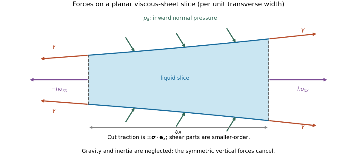
For force balance on the illustrated slice, the vertical cuts give $(h{\sigma }_{xx}{)}_x\delta x$. Pressure on the sloping broad faces gives $p_a{h}_x\delta x$ horizontally. Each of the two interfaces exerts a tangential surface tension pull at each cut, with horizontal component $\gamma \cos \theta$, where $\tan \theta =h_x/2$. Thus the horizontal force balance is the derivative of the effective tensionto the retained small-slope order. The ambient-pressure contributions cancel in this excess tension. Differentiating cancels the two $h_x{h}_{xx}$ terms, leaving the planar viscous-sheet stretching equationsThe upper-face kinematic condition is $w(x,h/2,t)=(h_t+u{h}_x)/2$. Combining it with $w=-z{u}_x$ gives the second equation,which is conservation of mass per unit transverse width.

For the two bubbles, let $p_g$ be the common gas pressure and $p_e$ the surrounding liquid pressure away from the sheet. A cylindrical bubble has one nonzero principal curvature, so the Young–Laplace equation gives $p_g-p_e\simeq \gamma /a$. In the nearly flat sheet the normal stress is $-p_g$, giving liquid pressure $p_{\mathrm{film}}=p_g-2\mu u_x$. The extensional correction is small compared with $\gamma /a$ because the transition scale will satisfy $\sqrt{a{h}_0}/L\ll 1$. Thus $p_{\mathrm{film}}\simeq p_g>p_e$, and this capillary pressure difference drives liquid out through both ends.

For a spatially uniform flat sheet, $h_x=h_{xxx}=0$, so the longitudinal equation gives $u_{xx}=0$. Reflection symmetry at $x=0$ selectsHere $U$ is the outward speed at the positive end. The mass equation then gives $h_t=-Uh/L$, independent of $x$, so initially uniform thickness remains uniform. Writing it as $h_0(t)$,The end transitions determine $U$, as derived in the following parts.

For an element $a$ of a complex unital Banach algebra, its spectrum of an element isThe nonzero spectra of products in opposite orders agree:For $\lambda \ne 0$, if $R=(\lambda 1-ab{)}^{-1}$ exists, direct multiplication on both sides verifiesInterchanging $a,b$ proves the converse. Zero may differ. On the Hilbert space ${\ell }^2({\mathbb{N}}_0)$, let $S$ be the unilateral shift operator $S{e}_n=e_{n+1}$ and take $a=S^{\ast }$, $b=S$. Then $ab=S^{\ast }S=I$, whereas $ba=S{S}^{\ast }=I-P_0$, where $P_0$ is projection onto the first coordinate. HenceBoth values for the second operator occur on its two nonzero invariant summands; every other value has an inverse obtained separately on those summands.

We use the spectral definition of a Positive element of a C-star algebra: $h$ is positive when $h=h^{\ast }$ and $\sigma (h)\subseteq [0,\infty )$. The continuous functional calculus, supplied by the Commutative Gelfand--Naimark theorem for the algebra generated by a Normal element of a C-star algebra and its adjoint, sends $F\in C(\sigma (h))$ to $F(h)$. It preserves products, sums, conjugation and the identity, is isometric, and satisfies $\sigma (F(h))=F(\sigma (h))$. For a self-adjoint element the spectrum is real, so real-valued functions produce self-adjoint elements.

For example, $F(t)=\sqrt{t}$ gives the positive square root in a C-star algebra of a Positive element of a C-star algebra. It satisfies $(h^{1/2}{)}^2=h$. Its uniqueness follows from the composition rule: if $d\ge 0$ and $d^2=h$, then the continuous functional calculus in the algebra generated by $d$ gives $\sqrt{d^2}=d$. For positive invertible $h$, the functions $t^{-1}$ and $t^{-1/2}$ give positive inverses and inverse square roots. If $0\le h$ and $r\ge \Vert h\Vert$, the function $r-t$ gives $r1-h\ge 0$; the same calculus givesThese transfer elementary scalar inequalities for functions of one element to the algebra. They do not justify applying a scalar inequality to arbitrary noncommuting elements.

To prove closure under addition without assuming an order theorem, let $a,b\ge 0$, set $\alpha =\Vert a\Vert$, $\beta =\Vert b\Vert$ and $s=\alpha +\beta$. If $s=0$, both elements are zero. Otherwise,The element $a+b$ is self-adjoint, so any $\lambda \in \sigma (a+b)$ is real and satisfies $|s-\lambda |\le s$. Thus $\lambda \ge 0$, provingWe will also use that the positive cone is proper: if $h\ge 0$ and $-h\ge 0$, then $\sigma (h)\subseteq \{0\}$, and the norm formula for self-adjoint elements gives $h=0$.

We next prove $a^{\ast }a\ge 0$ without presupposing that positivity is defined by such products. Put $h=a^{\ast }a$, which is self-adjoint, and form its negative part by the continuous functional calculus:This is positive. Let $c=a{h}_{-}^{1/2}$. Since $h_{-}$ commutes with $h$,The nonzero product-spectrum identity proved above gives $\sigma (c{c}^{\ast })\setminus \{0\}=\sigma (c^{\ast }c)\setminus \{0\}$. As $c{c}^{\ast }$ is self-adjoint, it too has spectrum in $(-\infty ,0]$, so $c{c}^{\ast }\le 0$.

Write $c=u+iv$ with $u=u^{\ast }$ and $v=v^{\ast }$. The continuous functional calculus makes $u^2$ and $v^2$ positive, and the addition result givesBut both summands on the left are nonpositive, so their sum is also nonpositive. Properness of the cone forces $c^{\ast }c+c{c}^{\ast }=0$. Now $c^{\ast }c=-c{c}^{\ast }$ is positive as well as nonpositive, so $c^{\ast }c=0$. The C-star identity gives $c=0$, whence $h_{-}^2=0$ and $h_{-}=0$. Thus $h$ has no negative spectral part:This proves the positivity of adjoint products from spectral positivity and the equivalence with the usual definition by elements of the form $d^{\ast }d$: the reverse direction is the factorization $h=(h^{1/2}{)}^{\ast }{h}^{1/2}$ for $h\ge 0$.

Finally, if $a\ge 0$ and $c\in A$, writeThe preceding result therefore provesIn particular, congruence preserves positivity in a C-star algebra, and $a\le b$ implies $c^{\ast }ac\le c^{\ast }bc$. These facts will justify the noncommutative order manipulations in the numbered parts.

A uniform algebra on a compact Hausdorff space $K$ is a closed complex subalgebra $A\subseteq C(K)$ containing the constants and separating points of $K$, with the supremum norm. It is therefore a commutative unital Banach algebra. Its character space of an algebra ${\Phi }_A$, also called its carrier space, consists of nonzero multiplicative linear functionals, equipped with the Gelfand topology.

For $x\in K$, evaluation gives the character of an algebra ${\delta }_x(f)=f(x)$. The map $\delta :K\to {\Phi }_A$ is continuous: composing it with the coordinate $\phi \mapsto \phi (f)$ gives the continuous function $f$ for every $f\in A$. It is injective because $A$ separates points. The Gelfand topology is Hausdorff because distinct algebra characters differ on some element of $A$. A continuous injection from compact $K$ into a Hausdorff space is a homeomorphism onto its image: closed subsets of $K$ have compact, hence closed, images. Its image is also compact and closed. Thusis the asserted homeomorphism. A natural uniform algebra is one for which this image is all of ${\Phi }_A$.